Part 6: Calculus | Year 11 Maths Advanced Guide – Free Worksheet

Struggling with Year 11 Calculus? In this Guide, we’re going to give you the rundown on what you need to know to ace Calculus and Year 11 Maths Advanced. We explain the concepts and then give you some examples to work through so you can track your progress.

Year 11 Advanced Mathematics: Calculus

Calculus plays an important role in building the foundation for later topics such as tangents and exponential growth and decay.

It is also an essential part in understanding the motions of a particle in the real world.

In this article, we’ll discuss

• NESA Syllabus Outcomes for Calculus
• Introduction to differentiation
• Utilising the chain, product, and quotient rules
• Finding stationary point(s) and determining the nature using the first derivative
• Finding the Displacement, Velocity and Acceleration Equations
• Concept check questions

NESA Syllabus Outcomes for Calculus

NESA dictates that students need to learn the following concepts to demonstrate proficiency in Calculus.

C1.3: The derivative function and its graph

• Establish that \(?′(?) = 0\) at a stationary point, \(?′(?) > 0\) when the function is increasing and \(?′(?) < 0\) when it is decreasing, to form a framework for sketching the derivative function.

C1.4: Calculating with derivatives

• Use the formula \(\frac{d(x^n)}{dx}=nx^{n-1}\) for all real values of \(?\)
• Understand and use the product, quotient and chain rules to differentiate functions of the form \(?(?)?(?), ?(?) ?(?)\) and \(?(?(?))\) where \(?(?)\) and \(?(?)\) are functions.
• Determine the velocity of a particle given its displacement from a point as a function of time.
• Determine the acceleration of a particle given its velocity at a point as a function of time.

Assumed Knowledge

Students should be familiar with limits, function notation and graphing non-linear functions.

Introduction to Differentiation

The most important concept to understand about differentiation is that the derivative is just a gradient. The same gradient that you learn in Year \(9\) with rise over run.

The only difference is that while in junior high school you’re finding the slope between \(2\) different points on a curve, the derivative tells you the slope at a singular point.

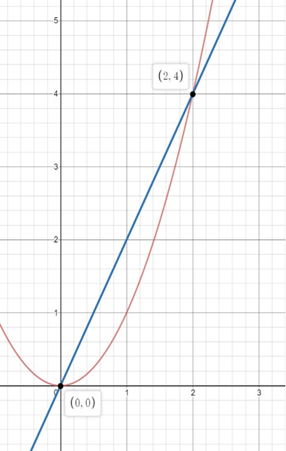
For example, to work out the slope between the \(2\) points above on the parabola \(y = x^2\), we would use rise over to run or our gradient formula to give \(m = \frac{4-0}{2-0}= 2\).

However, this simply gives us the average slope between those \(2\) points which we can see doesn’t correspond to the actual parabola. What if we wanted to find the actual curve of the parabola at a specific point such as \((2,4)\)?

If we were to use our normal gradient formula, it might look like the slope of the curve would be \(m =\frac{4-4}{2-2}=\frac{0}{0}\). This is where our derivative can be used.

What if we used the same concept of rise over run, but instead make it on a super, or infinitely small scale?

That would give us the slope of a curve at a specific point. Imagine we essentially zoom in on the point \([x, f(x)]\):

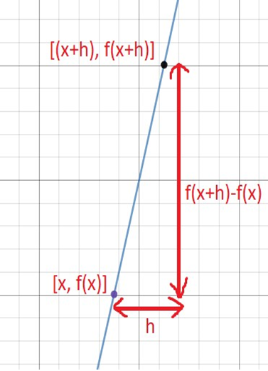
What we’ve done here is shrunk the size of our “run” to a very small value, which we name \(h\).

Now if we use the same gradient formula for this very small space, we’ll find that \(m = \frac{f(x+h)-f(x)}{x+h-x}\), which we can simplify to \(m = \frac{f(x+h)-f(x)}{h}\).
Now, if we want to find the gradient at the specific point \([x, f(x)]\), we let the value of \(h\) approach \(0\) since the gradient we’re looking for is at a single point. Doing this gives the result:

\(\frac{dy}{dx}=lim_{h→0}\frac{⁡f(x+h)-f(x)}{h}\).

This is what we call the first principles of differentiation.
Over the course of Year \(11\) and Year \(12\), you’ll learn other rules to differentiate different types of functions. One of the simplest ones is the derivative of power functions given by:

\(\frac{d(a\cdot x^n)}{dx}=a \cdot n \cdot x^{n-1}\)

Need help improving your Year 11 Maths Adv marks?

Learn from The HSC Experts with our Year 11 Maths Adv course. Learn more.

Utilising the Chain Rule, Product Rule and Quotient Rule

Chain Rule

Now that we know how to find the derivative of a function in terms of \(x\), such as \(f(x) = x^2-2x\), let’s consider how we would find the derivative of a composite function not necessarily in simple terms of \(x\), such as \(f(x) = (x+2)^2\).

One way we could do this question would be to expand the bracket and then differentiate normally.

However, we can also utilise chain rule as another method of differentiating \(f(x)\), which is given by:

\(\frac{dy}{dx}=\frac{dy}{du}\times\frac{du}{dx}\)

For our example here, we would let \(u=(x+2)\) and essentially set that as our new variable.

Going by the chain rule, we should have to work out what \(\frac{dy}{du}\) and \(\frac{du}{dx}\) are.

Now we can combine our two results to work out our derivative:

\begin{align*}
\frac{dy}{dx}=\frac{dy}{du}\times \frac{du}{dx} \\
=2\times (x+2) \times 1 \\
=2x+4
\end{align*}

Product Rule

We’ve talked about differentiating simple and composite functions, but what about the product of 2 separate functions?

For example, \(f(x)=(3x^2+4)×(9x-7)\).

Again, we can simply just expand the fraction in this case but later on the functions we get may become much more complicated and it may be easier to apply the product rule:

Quotient Rule

Our last differentiation rule we’ll be discussing is the quotient rule, which simply helps us find the derivative of a function that involves division or a fraction.

For example, \(f(x)=\frac{2x+7}{4x^3-7x}\).

The general rule formula for quotient rule is given by:

\(\frac{d}{dx} [\frac{f(x)}{g(x)}]=(f'(x)\cdot g(x) \cdot f(x) \cdot \frac{g'(x)}{[g(x)]^2}\).

Again, for simplicity, some may find it easier to replace \(f(x)\) and \(g(x)\) with \(u\) and \(v\) respectively, giving the same result:

\(\frac{d}{dx}(\frac{u}{v})=\frac{u’v-uv’}{v^2}\).

Finding stationary point(s) and determining the nature using the first derivative.

To understand both stationary points and their nature, let’s first understand what the derivative tells us about the curve’s behaviour:

Increasing

Condition: A positive derivative.
Example: \(y=x^3\)

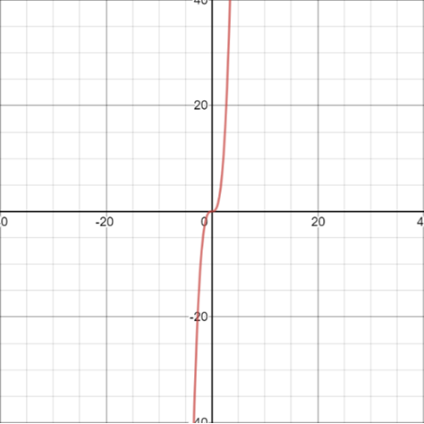
By differentiating, we get:
\(\frac{dy}{dx}=3x^2\)
Since the derivative is always positive, the curve must be increasing for all \(x\) values, which is shown in the adjacent graph.

Decreasing

Condition: A negative derivative.
Example: \(y=-x^3\)

By differentiating, we get:
\(\frac{dy}{dx}=-3x^2\)
Since the derivative is always negative, the curve must be decreasing for all \(x\) values.

Stationary Points

A stationary point is a point on the curve where it is neither increasing nor decreasing. Mathematically, these are the points that satisfy the following:
Condition: \(Derivative = 0\).

Minimum Stationary Point

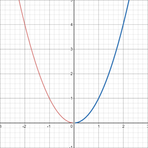
Conditions: \(\frac{dy}{dx}\) is negative to the left of the stationary point. \(\frac{dy}{dx}\) is positive to the right of the stationary point. A minimum stationary point at the origin will look as follows:

Maximum Stationary Point

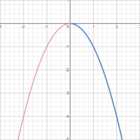
Conditions: \(\frac{dy}{dx}\) is positive to the left of the stationary point. \(\frac{dy}{dx}\) is negative to the right of the stationary point. A maximum stationary point at the origin will look as follows:

Consider the following process for finding stationary points and determining their nature:

Example 1

Find the stationary points of \(y=x^2+2x\)

Solution 1:

Step 1: Differentiate the equation.

\(\frac{dy}{dx}=2x+2\)

Step 2: To solve for stationary points, let \(\frac{dy}{dx}=0\).

\begin{align*}
2x+2=0 \\
2x=-2 \\
x=-1
\end{align*}

Step 3: When finding the \(y\)-coordinate of the stationary point, we substitute the \(x\) value back into the original function.

\begin{align*} y=x^2+2x \\
Let \ x= -1 \\
y=(-1)^2+2(-1)=-1 \end{align*}

Step 4: Determine the nature using a \(\frac{dy}{dx}\) table.

Setup the following table by:

• Plotting the \(x\) value of the stationary point in the middle.
• Choose an \(x\) – value that lies relatively close to the left and right of the stationary point.
• Find the \(\frac{dy}{dx}\) values at the chosen \(x\) – values.
• Determine whether it is a minimum or maximum.

Therefore, in this case, we have a minimum at \((-1, -1)\).

Finding the Displacement, Velocity and Acceleration Equations

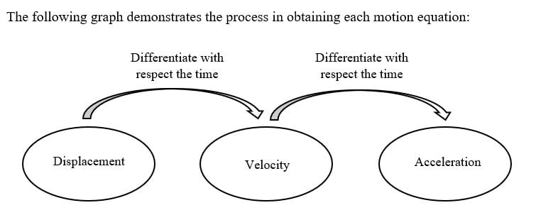
The following graph demonstrates the process in obtaining each motion equation:

Example 1:

Find the velocity and acceleration at \(t=5\) if the displacement equation is \(x=t^3+\frac{3}{t}\).

Solution 1:

To find the value of both velocity and acceleration, we must first find their equations.
Since we are given the displacement equation, in order to find the velocity equation, we must differentiate the displacement equation with respect to time.

\(v=\frac{dx}{dt}=3t^2-\frac{3}{t^2}\)

From our velocity equation, to get the acceleration equation, we must differentiate again with respect to time.

\(a=\frac{dv}{dt}=6t+\frac{6}{t^3}\)

Now to find both the acceleration and velocity at \(t=5\), we sub this into both equations.

\begin{align*}
v=3(5)^2 – \frac{3}{5^2} = \frac{1872}{25} \\
a=6(5) + \frac{6}{5^3} = \frac{3756}{125}
\end{align*}

Concept Check Questions

1. Differentiate the following using first principles:

(a) \(y=(x+2)^2\)
(b) \(y=3x+8\)

2. Find the gradient of the curve \(y=3x^3-x^2+8\) at the following points:

(a) \(x = 2\)
(b) \(x = -2\)

3. Differentiate the following functions:

(a) \(y=4x^4-2x^2+9x\)
(b) \(y=(x^2-8)(x-4)\)
(c) \(y=\frac{x^3-8x}{x^2+2}\)

4.  Find the stationary points of the curve \(y=8x^2-x^4\) and determine their nature.

5.  Given the displacement equation \(x=(t+3)^3+t^5\), find the velocity and acceleration at \(t=3\).

Concept Check Solutions

1.

(a) \(y’=2x+4\)
(b) \(y’=3\)

2.

(a) \(32\)
(b) \(40\)

3.

(a) \(16x^3-4x+9\)
(b)  \(3x^2-8x-8\)
(c) \(\frac{x^4+14x^2-16}{x^2+2}^2\)

4.

(a) Maximum: \((-2, 48), (2, 48)\)
(b) Minimum: \((0, 0)\)

5.

(a) \(Velocity = 513\)
(b) \(Acceleration = 576\)