Part 11: Variance and Standard Deviation | Year 11 Statistics

Are you confused about how to calculate and manipulate the variance and standard deviation for related sets of data?

You’re not the only one! In this blog post, we’ll cover the meaning of Variance and Standard deviation to help you prepare for Year 11 Advanced Maths.

Year 11 Advanced Mathematics: Statistics for Variance and Standard Deviation

Variance and standard deviation are measures of spread, extending upon your statistics knowledge from earlier years.

You will encounter the standard deviation again when considering probability distributions in year 12.

Additionally, a good understanding of standard deviation is key for using statistics appropriately after high school.

In this article, we’ll discuss:

• The NESA Syllabus Outcomes
• Measures of spread
• Variance for datasets
• Variance for discrete random variables
• Another way of calculating variance
• The standard deviation
• Sample vs population standard deviation
• Concept check questions
• Concept check solutions

NESA Syllabus outcomes:

NESA requires students to demonstrate proficiency in the following syllabus dot points:

S1.2: Discrete probability distributions

• use discrete random variables and associated probabilities to solve practical problems (ACMMM142) AAM
  • recognise the variance, \(Var(?)\), and standard deviation \((?)\) of a discrete random variable as measures of spread, and evaluate them in simple cases (ACMMM141)
  • use \(Var(X)=E((X-μ)^2 )=E(X^2 )-μ^2\)for a random variable and \(Var(x) = σ^2 \) for a dataset
• understand that a sample mean, \(\overline{x}\), is an estimate of the associated population mean \(?\), and that the sample standard deviation, \(?\), is an estimate of the associated population standard deviation, \(?\), and that these estimates get better as the sample size increases and when we have independent observations

Prerequisites

Students should be familiar with the definition of a discrete random variable; representations of discrete random variables; and mean and the expected value of a probability distribution.

If you need a refresher, check out our blog post on mean and expected value.

Measures of spread

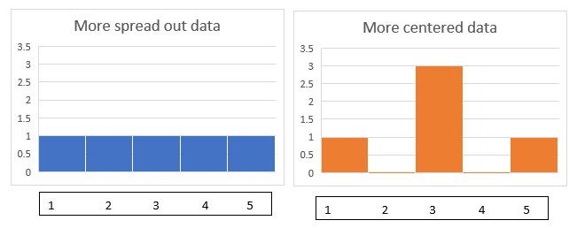
Consider these two sets of data:

\([1,2,3,4,5]\)

\([1,3,3,3,5]\)

They have the same mean \((3)\), same range \((4)\), and same median \((3)\). But they are different: the first set is more spread out, while the second one is more clustered towards the centre:

To summarise such differences, we use measures of spread, which are the range, Inter-quartile range (IQR), variance, and standard deviation.

Now, we’ve seen how the above two datasets have the same range, even though they are spread out differently.

We may similarly create two datasets with similar inter-quartile ranges but different spreads. The advantage of the variance and standard deviation is that it takes in information from all the data points, rather than just a few.

Variance for datasets

In earlier years, you may have used the following formula for variance:

\(Variance=\frac{\sum_{1}^{n}(x-\overline{x})^2}{n}\)

Let’s review the steps involved in the calculation above:

1. Find the mean,  \(\overline{x}\).
2. For each of the values in the data set, subtract the value from the mean, and take the square: \((x-\overline{x})^2\)
3. Add all these squares up: \(\sum_{1}^{n}(x-\overline{x})^2\)
4. Finally, divide by the number of values in the data set. \(\frac{\sum_{1}^{n}(x-\overline{x})^2}{n}\)

For our initial dataset, the process looks like this:

1. The mean of the dataset is \(\frac{1+2+3+4+5}{5} = 3\)
2. The difference from the mean of each of the data points is \([3-1,3-2,3-3,3-4,3-5] = [2,1,0,-1,-2]\). When squared, this gives up \([4,1,0,1,4]\)
3. The sum of the squares is \(4+1+0+1+4 = 10\)
4. Finally, dividing this by the number of values in the set \((5)\) gives us \(\frac{10}{5} = 2\). And that’s our variance!

Variance for discrete random variables

In Year \(11\) however, we will encounter discrete random variables, which don’t give us individual values for the dataset. Instead, we will encounter probability distribution tables, like the one below:

Recall that this means that there is a \(1\) in \(10\) chance of \(x\) being \(1\), a \(1\) in \(4\) chance of \(x\) being \(2\), and so on.

Since we don’t have individual numbers, we must use a different formula for calculating the variance.

Previously, we divided by the \(n\), number of elements in our dataset to get the variance, because the chance of getting each value was \(\frac{1}{n}\).

Now that the probability is different, we need to use the expected value of the difference from the mean.

If we also notice that the mean is \(\overline{x}=μ=E(x)\) when we have a probability distribution table, then we can use the following steps:

1. Find the expected value of the original probability distribution table, \(μ=E(x)\).
2. Subtract each value in the probability distribution from the mean: \(x-μ\)
3. Square each of the differences, as we did before: \((x-μ)^2\)
4. Take the expected value of these squares, by multiplying by the probability corresponding to each value from the table; and then add them up: \(E((x-μ)^2)\)

And that’s it! The formula for variance is

Using the process above on the table above, we have:

1. The mean is \((0.1+0.5+1.2+1.5+0.5) = 3.8\)
2. Subtracting each of the values from the mean, we get: \([2.8,1.8,-0.2,-1.2,-6.2]\)
3. Squaring these, we get: \([7.84,3.24,0.04,1.44,38.44]\)
4. Multiplying by the respective probabilities, and summing the data, we get a variance of \(3.96\)

Another way of calculating variance

Revisiting the formula:

We can rearrange our equation to obtain another way to calculate the variance.

\begin{align*}
E((x-μ)^2)=\sum_{1}^{n}(x-μ)^2p(x) \\
=\sum_{1}^{n}(x^2-2xμ+μ^2)p(x) \\
=\sum_{1}^{n}x^2p(x)-μ \sum_{1}^{n}xp(x)+\sum_{1}^{n}p(x)μ^2 \\
=E(x^2)-μ^2
\end{align*}

The significance of this result is that if you are given only the mean μ and the expected value of the square \(E(x^2)\), you can still calculate the variance. You can also use it to check your answers whenever a variance question pops up.

The standard deviation

One issue with the variance as a measure of spread is that it does not scale linearly with a dataset. Consider what happens if we double our initial dataset:

We might think that the spread should double, since we have doubled our dataset. But what is the variance of this dataset?

Our original variance was \(2\), so this time the variance has increased by \(4\) times. So if we double our dataset, our variance increases by \(4\) times; and if we triple our dataset, our variance will increase by \(9\) times, and so on.

This means that comparing variance in very large data sets may be difficult. How can we even out this difference?
We can try taking the square root of our variance, and this is called the standard deviation.

So, our standard deviation for our original data set is \(std.dev=\sqrt2\), and our standard deviation for our doubled data set is \(std.dev=\sqrt8=2\sqrt2\). This is double our original standard deviation, so it seems we are on the right track. Now let’s check against our second data set, when doubled:

\(New \ dataset=[2,6,6,6,10]\)
\(New \ Variance=\frac{(-4)^2+0+0+0+4^2}{5}\)
\(=\frac{32}{5}=6.4\)
\(New \ std.dev=\sqrt6.4=2\sqrt1.6\)

And our old variance was \(1.6\), which means our old standard deviation was \(\sqrt1.6\) which is half of our standard deviation for our doubled second set. The standard deviation scales the same way as our data, making it a useful statistic to measure.

In general, you can obtain the standard deviation by taking the square root of the variance, even if you are dealing with probability distributions instead of data sets:
\(Standard \ deviation=σ=\sqrt(Variance)\)

Standard deviation will appear again in year \(12\) when looking at continuous distributions, so make sure you’re comfortable with the concept!

Sample standard deviation

Just like the sample mean, a sample standard deviation exists for samples of a population, if you are not given data or a probability distribution for the full population. Do note that you do not need to know the formula for the sample standard deviation for the HSC, but you should be aware that it is different from (it is an approximation of) the population standard deviation.

The sample standard deviation gets closer to the population standard deviation (and hence is more accurate) if:The sample standard deviation gets closer to the population standard deviation (and hence is more accurate) if:- Your samples are independent of any external factor / preference- Your sample size is larger.

Want to remove the variance from your Year 11 Maths Advanced results?

Matrix+ online Year 11 Maths Advanced courses are the expert guided solution to your Maths problems. Learn more now!

Concept check questions

1. What is the variance of the following probability distribution?

2. Given the standard deviation of a dataset is \(5\), what is the variance of the dataset?

3. If the variance of a dataset is \(16\), and the expected value of the squares of the dataset is \(22\), what is the mean of the dataset?

Concept check solutions

1. The following table can be used to calculate the variance:

Then \(E(x) = 1.5+2.4+2.1 = 6.0\), and \(E(x^2)=36.6\), giving us a variance of \(0.6\).

2. The variance is the square of the standard deviation, which is \(25\).

3. Since \(Variance = E(x^2) -μ^2, μ^2=E(x^2 )-Variance = 22-16 = 6\). The mean is therefore \(\sqrt6\).