Welcome to Matrix Education
To ensure we are showing you the most relevant content, please select your location below.
Select a year to see courses
Select a year to see available courses

So you know how to solve continuous random variables and functions, but you’re still unsure about normal distribution. Don’t worry! This article will guide you through everything you need to know about normal distribution.
Try our free worksheet!
A worksheet to test your knowledge. 
Free Year 12 Normal Distribution Worksheet Download
When scientists began taking rigorous statistical measurements of natural phenomena, a number of common patterns emerged. Of these, the most common distribution had sample values deviating from a mean value in predictable proportions.
This makes the so called “normal distribution” a useful tool to study and compare data sets with.
This blog article will explain the Normal Distribution and several properties of the normal distribution that can be applied to various data sets.
This resource will help by supplementing the new Year 12 Syllabus to provide an introduction or a refresher on the Normal distribution.
S3.2: The normal distribution
Students:
To understand the normal distribution, you should have a good understanding of:
Need a refresher on continuous random variables? Check out our post on Continuous Random Variables.
The Normal Distribution is a common distribution of a continuous random variable.
A quick refresher: A distribution of a continuous random variable describes the probability that a given variable (whether measured or chosen out of an existing dataset) will fall in a certain range.
A normal distribution is distinguished from other probability distributions by its particular shape:
A binomial distribution
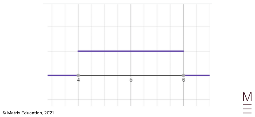
A uniform distribution
Normal distributions are typically suitable for measurements of a physical quantity e.g. height or weight in a population where there is some variation.
Typical examples of normal distributions might be the height of a class of students, or the weight of a population of marmots.
The normal approximation may also be applied to financial models, for example in the stock market.
When describing the shape of the Normal Distribution, we note that the shape is symmetrical about the mean.
Although all normal distributions have the same shape, they can be shifted or stretched to fit different sets of measurements depending on two key parameters.
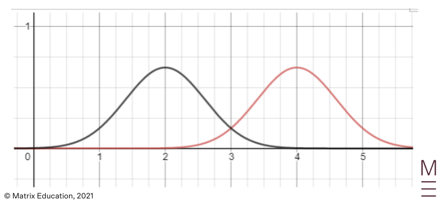
The mean of the measurements determines where the peak (also the centre) of the normal distribution lies.
The mean is usually denoted using the symbol \( \mu \).
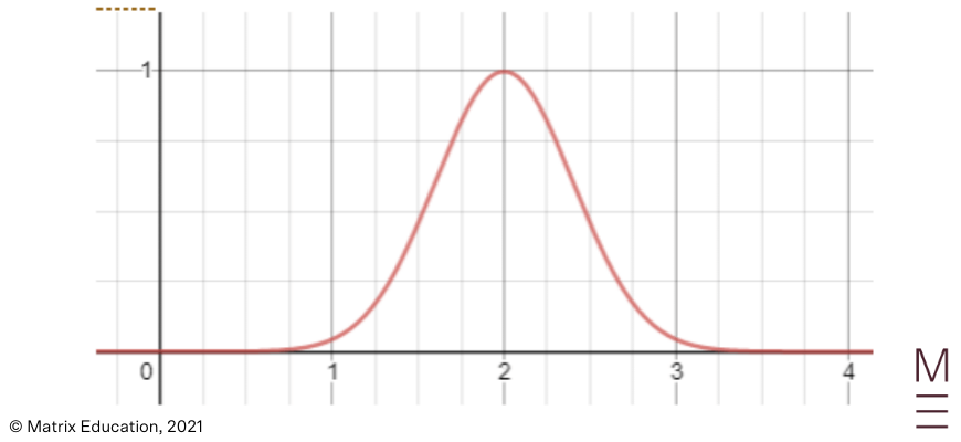
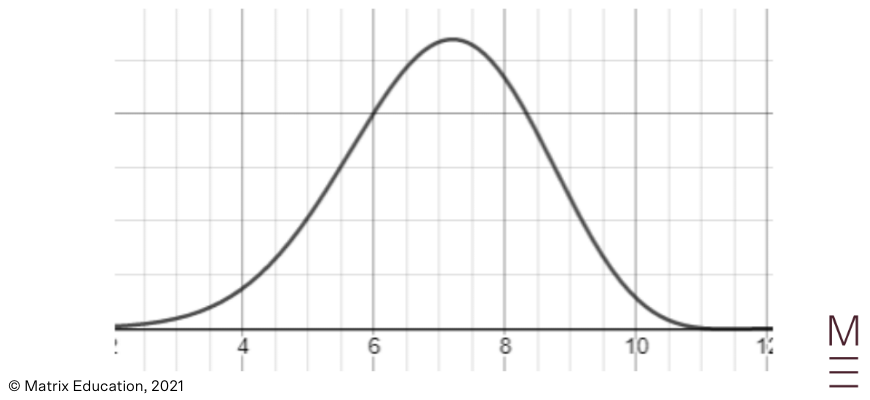
For example, in the graphs below, the first curve has a mean of 2 and the second has a mean of 4.
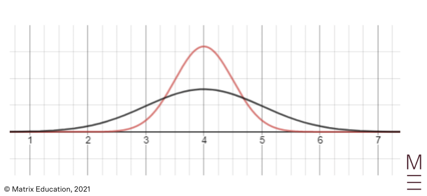
The standard deviation of the measurements determines how flat the normal distribution is.
The standard deviation is typically denoted using the symbol \( \sigma \)..
A high standard deviation results in a flatter curve, compared to a lower standard deviation.
For example, in the graphs below, the red curve has a standard deviation of 0.5 and the black curve has a standard deviation of 1.
Both are still normally distributed however!
A function can be derived for the normal distribution using calculus.
Formally, a normal distribution is one in which the likelihood of a value occurring decreases proportional to the distance between the mean and the value, and also decreases proportional to the likelihood itself.
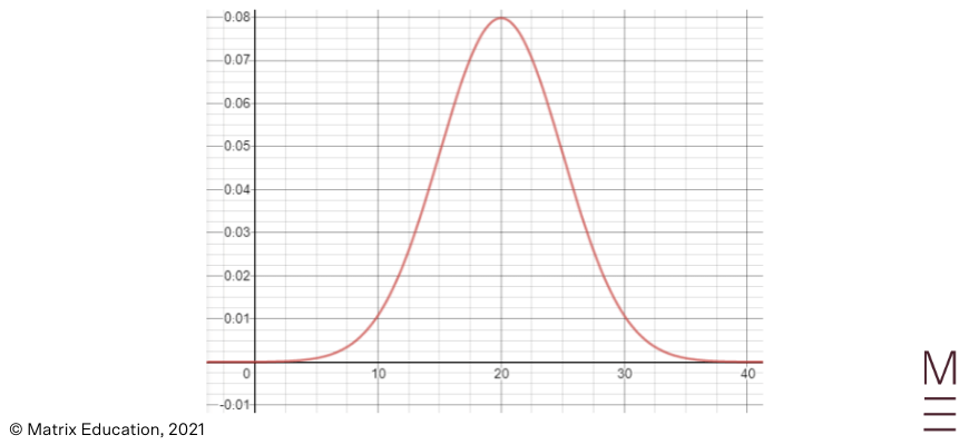
This results in a differential equation which can be solved to produce the following probability density function (the derivation of which is typically covered in university):
If you use Desmos or another graphing calculator to plot the function above (specifying \( \sigma \) and \( \mu \), you will get the normal distribution curve as seen in the screenshots above.
If we have a normally distributed set, how can we quickly compare how far a point is from the centre?
Say we have a point that is 10 from the centre. This would be a lot if the standard deviation was 1; but would be relatively small if the standard deviation was 100.
For this reason, we should adjust the distance from the centre by the standard deviation by dividing by the standard deviation.
This results in the z-score, which is given by the formula:
\( z – score = \frac{x-\mu}{\sigma} \)
Where \( x \) is a particular data point, \( \sigma \) is the standard deviation, and \( \mu \) is the mean.
Note that this means if the value is bigger than the mean, then the z-score is positive; but for values less than the mean the z-score will be negative.
Since the standard deviation has the same shape but is flattened by the standard deviation, when we divide by the standard deviation, this reverses the flattening effect for the single data point.
Therefore, we can use the z-score to make inferences about the particular data point based on the general shape of the normal distribution.
A given z-score corresponds to a given rarity; and for z scores of 1, 2 and 3, we have:
| z-score | Percentage of values that are less than that z-score |
| +1 | 68% |
| +2 | 95% |
| +3 | 99.7% |
This set of z-scores should be remembered, and collectively they are known as the Empirical rule.
Be prepared to interpret similar tables as well in an exam!
After a haircut, a curious student collects their hair and finds that the lengths of the hair follow the normal distribution. The mean hair length is 20cm, and the standard deviation is 5cm.
1.
2.
a. False: Even though the mean is 20, there do not have to be any hairs that are exactly 20cm long.
b. True: The interquartile range is the range between 25% and 75% probability; and we know that 75% is between 1 z-score and 2 z-score, i.e. between 25 and 30. Similarly, 25% is between -1 z-score and -2 z score, i.e. between 15 and 10. Therefore, the interquartile range is at most 30-10=20cm.
c. False: although it is highly likely that no hair is longer than even 40cm, there is a possibility that there is a hair that is 50cm long.
3. The z-score is \( \frac{18-20}{5} = \frac{-2}{5} = -0.4 \)
4. 10 corresponds to a z-score of -2. We know that 95% of hairs are shorter than 2 z-scores more than 20cm; and because of symmetry, 95% of hairs are longer than -2 z-score. This leaves 5% of hairs less than 10cm.
5. Again, because of symmetry, we have just as many hairs that are more than \( z = \frac{22-2}{5} = 0.4 \) away from the mean, as there are hairs that are less than \( x = \mu – 0.4 \sigma = 20 – 2 = 18 \) cm.
Gain confidence in all of your core Maths Adv topics before your HSC! Our HSC Exam Prep Course will help you revise and break down these core topics, and provide you with plenty of practice questions and papers to help you develop your exam-taking skills. Learn more about the HSC Prep Course now.
© Matrix Education and www.matrix.edu.au, 2025. Unauthorised use and/or duplication of this material without express and written permission from this site’s author and/or owner is strictly prohibited. Excerpts and links may be used, provided that full and clear credit is given to Matrix Education and www.matrix.edu.au with appropriate and specific direction to the original content.