Part 3: Linear Regression | Free Worksheet

Still unsure about linear regressions and bivariate data? Well, don’t fear! We will explain everything you need to know to ace linear regressions.

In this article, we’ll discuss:

• The NESA Syllabus Outcomes
• Bivariate Data:
  • Scatter Plots
  • Linearity
  • Correlation
• Pearson’s Correlation Coefficient
• Line of best fit
  • Interpolation and Extrapolation
• Concept Check Questions and Solutions

Check your linear regression skills!

Year 12 Advanced Mathematics: Bivariate Data Analysis

Probability and Statistics is extensively used in mathematics, statistics, finance, science, artificial intelligence and many more areas of study.

Surprisingly, the topic that underpins hard probability problems is an area of mathematics called combinatorics (meaning counting!) Indeed, as probabilities are the ratios of the number of ways an event can happen to the total number of possibilities, the step is to develop a theory of counting.

We are going to look at the following NESA syllabus points.

NESA Syllabus Outcomes

The following Syllabus Outcomes will be addressed in this Subject Guide:

• Construct a bivariate scatterplot to identify patterns in the data that suggest the presence of an association
• Use bivariate scatterplots (constructing them where needed), to describe the patterns, features and associations of bivariate datasets, justifying any conclusions
  • Describe bivariate datasets in terms of form (linear/non-linear) and in the case of linear, also the direction (positive/negative) and strength of association (strong/moderate/weak)
  • Identify the dependent and independent variables within bivariate datasets where appropriate
• Calculate and interpret Pearson’s correlation coefficient (r) using technology to quantify the strength of a linear association of a sample
• Model a linear relationship by fitting an appropriate line of best fit to a scatterplot and using it to describe and quantify associations
• Interpret the intercept and gradient of the fitted line
• Use the appropriate line of best fit, both found by eye and by applying the equation of the fitted line, to make predictions by either interpolation or extrapolation
  • Distinguish between interpolation and extrapolation, recognising the limitations of using the fitted line to make predictions, and interpolate from plotted data to make predictions where appropriate
•  Solve problems that involve identifying, analysing and describing associations between two numeric variables

Assumed Knowledge

Students only need to be familiar with arithmetic for combinatorics.

Students should already be familiar with the basic concepts of probability. They should also understand basic algebraic techniques and expansion to understand the concepts explored in the following guide.

Bivariate Data Analysis

Bivariate Data is data collected in pairs \( (x, \ y) \) being the results of some experiment or observation.

Here, the variable is called the \( x \) independent variable and the variable \( y \) is called the dependent variable.

For example, \( x \) may be the amount of money invested in TV advertising for a particular business and \( y \) can be the corresponding profit that business earnt for that value of \( x \).

For instance, a data point would mean $2500 was invested in advertising, and $7000 was made in profit.

In Bivariate Data analysis, we aim to see if there is a relationship or an association between the variable \( x \) and \( y \). This relationship will generally be just a trend, and not a deterministic relationship, because the variable \( y \), like profit in the above example, may depend on may other factors not captured by just \( x \).

Now, we will introduce some terminology and tools used to describe bivariate data.

Scatter Plots

Bivariate data can be visualized using a scatter plot, where the independent variable is placed on the horizontal axis, and the dependent variable is placed on the vertical axis.

Linearity

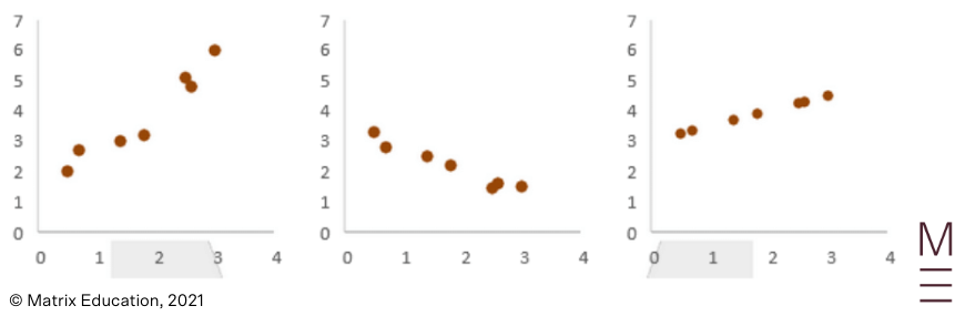
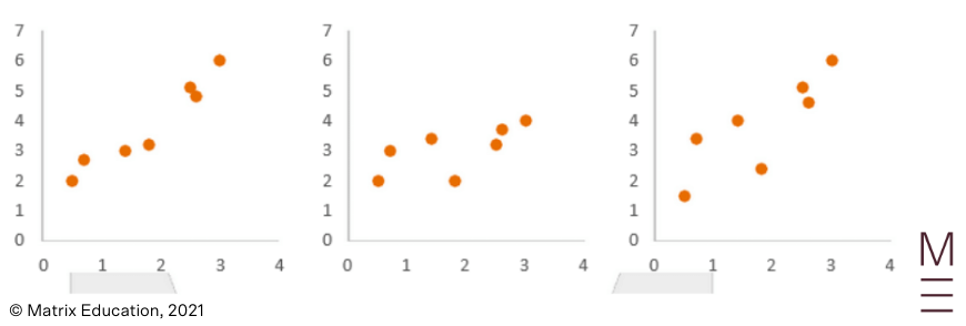
A dataset is linear if the data has a roughly linear trend. For instance, the following plots indicate a linear dataset:

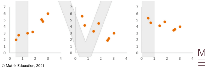
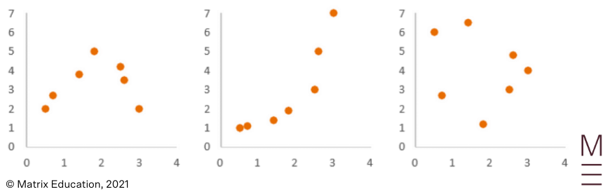
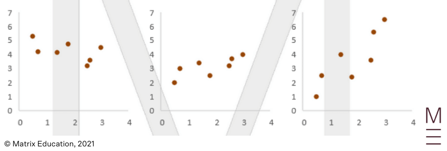
A data set is non-linear if the data does not follow a line shape. Instead, it could have no trend at all, or perhaps a curved/more complicated trend.  For instance:

Correlation

The correlation measures the strength and direction of this linear relationship. We will look at each of these below:

Strength

When there is a linear trend, the strength of association can be of three categories – strong correlation, medium correlation and weak correlation. When there is no linear trend, we say there is no correlation. The strength of correlation is to do with how aligned the data points are.

Strong Correlation: The following plots exhibit strong correlation.

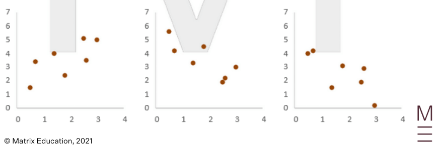
Medium Correlation: The following plots exhibit medium correlation.

Weak Correlation: The following plots exhibit weak correlation.

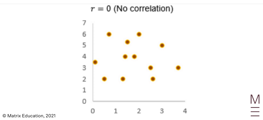
No correlation: We can also have no correlation, meaning the data points show no sign of linearity.

Direction

Correlation can be positive or negative.

Positive Correlation: The following plots exhibit positive correlation – as \( x \) increases, \( y \) increases.

Pearson’s Correlation Coefficient

So far, we have only described correlation qualitatively. However, it is difficult to compare two plots which both might have medium strength positive correlation.

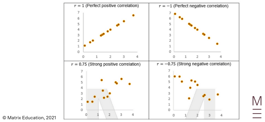
Pearson’s correlation coefficient is a quantitative measure for correlation. It denoted by the letter \( r \) (which is why it is also called Pearson’s \( r \) ) and ranges between -1 and 1.

The magnitude of Pearson’s coefficient relates to the strength of the linear relationship. The sign of Pearson’s coefficient describes the direction of the linear relationship.

The following plots are annotated with how to interpret Pearson’s correlation.

Line of best fit

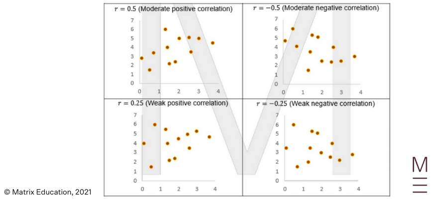
As we have seen, while our data on a scatter plot may not be exactly linear, there may be a linear trend. We can describe this linear relationship qualitatively or using Pearson’s Coefficient.

Now, we will actually approximate the data using a line of best fit (also know as the least-squares regression line). A line of best fit aims to best represent the data at hand with a straight line.

When a line of best fit is constructed by a computer or by a calculator, the line drawn will have the shortest vertical distance from the data points as possible.

There are various reasons to use a line of best fit:

• It summarises the data points into an approximate relationship between \( x \) and \( y \)
• We can interpret the features of this line (such as the intercept and the gradient)
• We can use the line to make predictions (through interpolation and extrapolation)

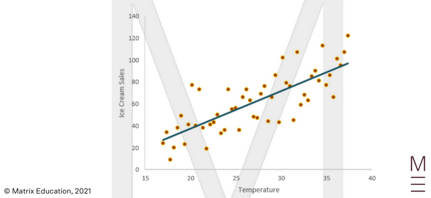
Students need to be able to draw an approximate line of best fit. For example, the line of best fit through the below scatter plot is shown:

Using the Calculator

The syllabus requires students to use technology to find

• The Pearson’s Correlation Coefficient \( r \)
• The Equation of the Line of Best Fit \( y = A + Bx\)

when data is provided. In exams, they can use their calculators to do so.

Steps:

1. Clear your Calculator from any previous data entries (SHIFT \( \rightarrow \) 9 \( \rightarrow \) 3)
2. Select linear regression in your Calculator from “STAT” mode (MODE \( \rightarrow \) 2 \( \rightarrow \) 2)
3. Input your Data and then press AC when you are finished
4. To retrieve the Correlation Coefficient or the Parameters A and B of your line, press SHIFT \( \rightarrow \) 1 \( \rightarrow \) 5 and then select either 1, 2 or 3 depending on what you are after.

Interpolation and Extrapolation

Once the line of best fit is drawn, calculated or provided by the question, it can be used to predict the value of \( y \)  at a hypothetical value of \( x \) .

• If we have hand-drawn the line of best fit, we can approximate the \( y \) value at the hypothesised value of \( x \)
• If an equation of a line of best fit is provided, we can substitute the hypothesised value of  \( x \) into the equation to approximate the value of \( y \).

There are two types of prediction:

• Interpolation: Predicting \( y \) for a value of \( x \) inside the range of our data
• Extrapolation: Predicting  \( y \) for a value of \( x \) outside the range of our data

Here, the range of our data refers to the  values between the first point and the last point as you go from left to right.

Note: Extrapolation is prone to error because it assumes the trend in the existing data will continue for values of \( x \) outside of the data available. Unless the data analyst is sure that the linearity of the trend will continue instead of, for example, curving off, extrapolation can produce meaningless data because of the strong assumptions.

Concept Check Questions

The CEO of a company wanted to see the relationship between the number of years that each employee has been working for and their annual salary. The results are displayed in the scatterplot below:

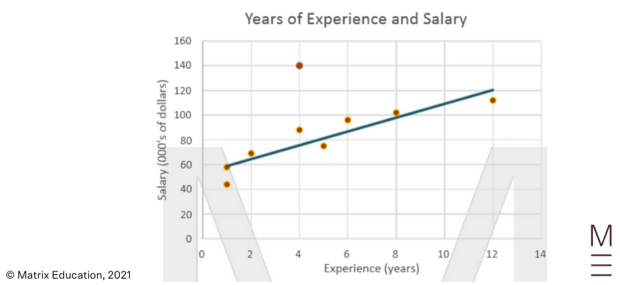
1) Identify any outliers.

2) Estimate the correlation coefficient.

3) What is the equation of the least squares regression line?

4) What is the meaning of the intercept and gradient of this model?

5) Matthew has been working at the company for 10 years. Predict his salary.

Concept Check Solutions

1) The point (4, 140) is an outlier, potentially an exceptional employee that is compensated highly for their work despite having less experience than others.

2) 0.9 (The data is fairly linear and positively correlated)

3) \( y = 5.25x + 58 \)

4) The intercept approximates the average salary of an employee with no experience to be around $58,000 while the gradient suggests a $5250 increase in annual salary from a one-year increase in experience.

5) $110,000

Watch your marks rise in a strong and positive trend

Learn Maths Adv from home with Matrix+ Online Course! We will provide you with video theory lessons, access to our comprehensive Maths workbooks mailed to your door, and Q&A Discussion Boards to help you target your questions. Learn more about Matrix+ Online Maths Adv Course now.