Part 4: Continuous Random Variables | Free Worksheet

Are you still rusty with continuous random variables? Well, you came to the right place! We will explain what a continuous random variable is, and show you how to interpret different types of functions.

In this article we’ll discuss:

• The NESA syllabus outcomes
• Assumed knowledge
• What is a continuous random variable?
• Interpreting histograms
• The probability density function
• Interpreting the probability density function
• Cumulative distribution functions
• Concept Check Questions

How well can you apply your knowledge of continuous random variables?

Test your knowledge with our free worksheet.

Download your free Continuous Random Variables worksheet

This worksheet has 4 levels of difficulty to test your knowledge

Download now     

Done! Your download has been emailed.

Please allow a few minutes for it to land in your inbox.

School Year in 2023

7

8

9

10

11

12

Send it to me!

We take your privacy seriously. T&Cs and Privacy Policy.

Year 12 Advanced Mathematics: Continuous Random Variables

In today’s Big Data world, an understanding of statistics is particularly important to make the best use of the data collected. With such large volumes of data, individual data points can be approximated by random variables, allowing for a simplification of modelling that can be used to sense-check a course of action.

This blog article will explain Continuous Random Variables and several techniques that can be used to analyse a set of continuous random variables.

This resource will help by supplementing the new Year 12 Syllabus to provide an introduction or a refresher on the topic of Continuous Random Variables.

NESA Syllabus outcomes

S3.1: Continuous random variables

Students:

• Use relative frequencies and histograms obtained from data to estimate probabilities associated with a continuous random variable- Understand and use the concepts of a probability density function
  • Know the two properties of a probability density function: \( f(x) \geq 0  \) for all real \( x  \) and \(  \int_{-\infty}^{\infty} f(x) \ dx = 1 \)
  • Define the probability as the area under the graph of the probability density function using the notation \( P (X \leq r )= \int_{a}^{r} f(x) \ dx\), where \( f(x) \) is the probability density function defined on \( [a,b] \)
  • Examine simple types of continuous random variables and use them in appropriate contexts
  • Explore properties of a continuous random variable that is uniformly distributed
  • Find the mode from a given probability density function
• Obtain and analyse a cumulative distribution function with respect to a given probability density function
  • Understand the meaning of a cumulative distribution function with respect to a given probability density function
  • Use a cumulative distribution function to calculate the median and other percentiles

Assumed Knowledge

In Year 11, you would have learnt about:

• What a random variable is
• The difference between a discrete and a continuous random variable
• Probability distribution tables
• Constraints on probability distributions (e.g. \( \sum p(x) = 1 \))
• The definition of some common terms in statistics, including mean, median and mode

You should also be comfortable with practical applications of calculus, including

• Finding the maximum value of a function
• Interpreting the integral of a function as the area under its curve.

These concepts and terms will be extended upon in the following sections about continuous random variables.

What is a continuous random variable?

In Year 11, you constructed probability distribution tables for numerical, but discrete, random variables.

Compared to discrete random variables, which can only take on a set of values, continuous random variables can take on an infinite number of numerical values.

For example, if you have 5 lollies to put in two bags, either bag can only have 0, 1, 2, 3, 4 or 5 lollies.

However, if you had 5 litres of water to pour into two containers, a container can hold any range from 0 to 5 litres, including 0.1 L, 3.74 L, or 4.99 L.

This makes it difficult to calculate statistics using probability distribution tables, since there are infinite possible values!

Fortunately, you have already learnt some tools with dealing with infinite divisions, namely Calculus.

We can also group various ranges of values in bins to produce a frequency histogram.

Interpreting histograms

Histograms are one way to simplify continuous random variables.

In a histogram, data points are sorted into various bins, and those bins are then graphed.

Consider the following data:

If we group them in groups from 0 – 5, 5 – 10, 10 – 15, 15 – 20, 20 – 25, 25 – 30, we have the following tally:

From this tally we can generate the histogram below:

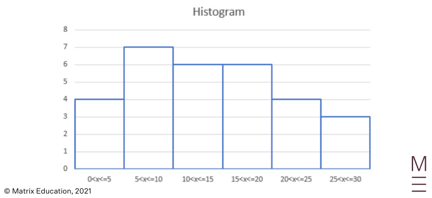
You may be asked to read a histogram to determine the relative percentage of values that fall within a given range; or asked to construct a histogram from a given data set.

Want to test your knowledge of continuous random variables?

[InlineContentDownloadForm]

The probability density function

When the number of data points gets larger, it may become infeasible to count how many values are in each group.

Additionally, even though an event is random, there may be rules that govern the outcome of the event.

This is formalised as a probability density function \( f(x) \), which is defined as:

There are two important properties you need to know about the probability density function.

Firstly, remember from Year 11 that the sum of all probabilities in a probability distribution table is 1, because the random variable must take on a value in the probability distribution table.

Similarly, if we extend the range \( (a,b) \) to all possible numbers (i.e. \( (a,b) = (- \infty, \infty) \), then the outcome must fall within this range; so it follows that

Secondly, the probability of an event occurring must not be negative, so all values of \( f(x) \geq 0 \).

The shape and definition of \( f(x) \) can vary greatly but will be specified in the question.

However, one probability definition you should know how to interpret is a uniform probability distribution.

A uniform probability distribution can be represented as a piecewise function:

$$
f(x)=
\begin{cases}
\frac{1}{b-a} & ;a \ \leq \ x \ \leq \ b \\
0 & ;otherwise
\end{cases}
$$

That is, within some range, the probability is constant; outside the range, the probability is zero.

Interpreting the probability density function

We can interpret the probability density function to derive some useful results.

Consider a large population of rabbits, whose ear length is given by some probability distribution function \( f(x) \).

If we are asked, what is the probability that a selected rabbit has an ear length of under 10cm, we could express our answer in terms of the probability density function:

 \( P(X \leq 10) = \int_{-\infty}^{10} f(x) \ dx \)

What if we were asked to find the mode of the ear lengths?

Recall that the mode of a distribution is the most likely value.

However, since it is incredibly unlikely that even two rabbits have the exact same ear length as the range is continuous, we need to redefine our mode.

Thus, the mode of a continuous random distribution is the value of \( x \) for which the function \( f(x) \) is maximised.

This can be found by solving for \( f'(x) = 0 \), as per the standard method of solving for the maximum value of a function.

Cumulative distribution functions

If you were asked to find the median value of the continuous random variable, you would need to find the value below which 50% of the data points lie.

However, our probability distribution function only allows us to answer questions which take a value and gives us a proportion, by setting the bounds of the integral \( \int_{a}^{b} f(x) dx \).

To answer the median question, then, we need to create a cumulative distribution.

The cumulative distribution function is the proportion of values that are lower than a certain value \( X = v \).

This can be found by changing the variable in our integral to the bounds of the integral,

i.e.

.

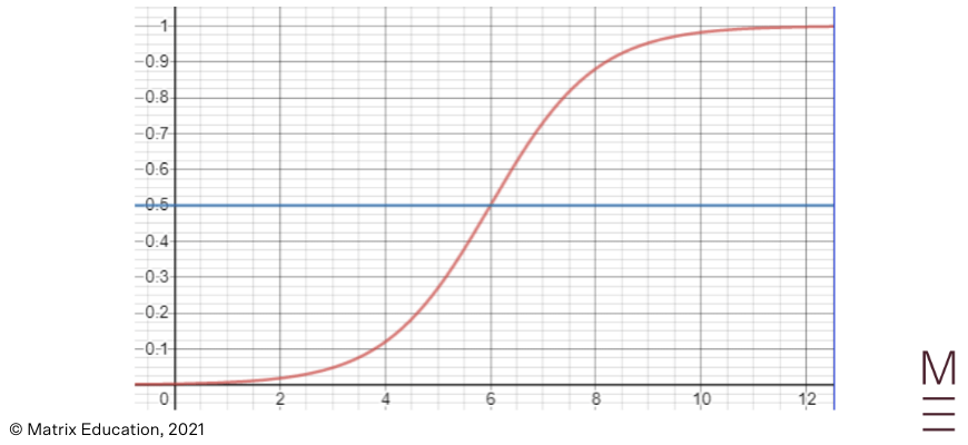
A cumulative distribution function will start from 0 at \( x = -\infty \) and end at 1 at \( x = \infty \), as no value is smaller than negative infinity and no value is bigger than positive infinity.

Additionally, a cumulative distribution function will never be decreasing, as the value at any point represents the total proportion of values up to and including those less than it.

Given a cumulative distribution function, we can find the median by:

1. Graphing it (with the x-axis being the value and the y-axis being the probability);
2. Drawing a line at y = 0.5 (50% of the values);
3. Reading off the x-value.

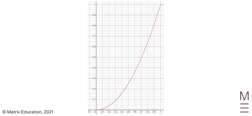
In the above example, the median is 6.

We can similarly find other percentiles by drawing other horizontal lines and reading off the x-axis.

For example, to find the 30th percentile, we would draw a line at y = 0.3.

Concept check questions

1. Consider the following histogram describing the intensity of solar flares over a period. The histogram has been normalised to show probability values rather than the total count.

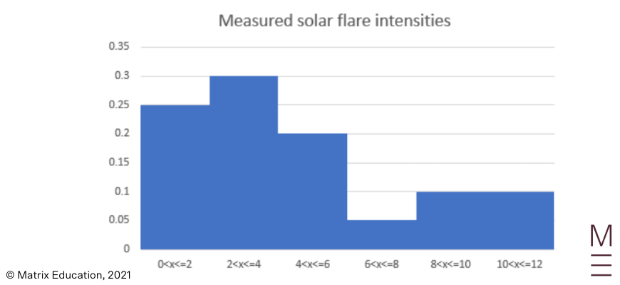
a. What is the probability that the measured intensity is below 4?

b. What is the probability that the measured intensity is above 6?

2. Using the above histogram, a scientist makes the following statements. Which are valid?

a. “The proportion of solar flares with between 6 and 7 intensity is 0.025.”

b. “The median solar flare intensity is between 2 and 4.”

3. Determine whether the functions below are valid probability distribution functions:

a. $$
f(x) = x^2
$$

b. $$
f(x)=
\begin{cases}
\frac{1}{5} & ;4 \ \leq \ x \ \leq \ b \\
0 & ;otherwise
\end{cases}
$$

c.$$
f(x)=
\begin{cases}
x & ;-1 \ \leq \ x \ \leq \ \sqrt{3} \\
0 & ;otherwise
\end{cases}
$$

d. $$
f(x)=
\begin{cases}
1 & ;x = 5 \\
0 & ;otherwise
\end{cases}
$$

4. A [phenomenon] can be described using the following probability distribution function:

$$
f(x)=
\begin{cases}
\frac{3x^{2}}{19} & ;2 \ \leq \ x \ \leq \ 3 \\
0 & ;otherwise
\end{cases}
$$

What proportion of samples taken will be:

a. Less than 2?

b. Less than 2.5?

c. Greater than 2.7?

5. A cumulative distribution function is provided below:

a. What is the median of the distribution?

b. What is the 25th percentile?

c. What is the 75th percentile?

d. The function is always concave up between 0 and 1. What is the mode?

Concept check solutions

1.

a. The probability that the measured intensity is below 4 is 0.25 + 0.3 = 0.55.

b. The probability that the measured intensity is above 6 is 0.05 +0 .1 + 0.1 = 0.25.

2.

a. This statement is not correct as we cannot know the distribution of a part of the samples.

For example, it’s possible that between 6 and 7 the probability is 0.04 and between 7 and 8 the probability is 0.01.

b. This statement is true, since the median is defined at the point where half the values (0.5) are below; and this lies somewhere between 2 and 4 (although we don’t know exactly).

3. 

a. No, this is not a valid probability distribution function; since the integral \( \int_{-\infty}^{\infty} x^{2} = \infty \neq 1 \)

b. Yes. This is a uniform distribution between 4 and 9.

c. No, this is not a valid probability distribution function, as although it integrates to 1, there are negative probabilities which are not allowed.

d. Yes. This is a variant on a common probability distribution function in physics known as the Dirac delta function.

4.

a. 0, since the probability distribution function is 0 for all values below 2.

b.

c.

5. 

a. At \( y = 0.5, x = 7.125.\)

b. At \( y = 0.25, x = 0.5.\)

c. At \( y = 0.75, x = 8.625.\)

d. If the function is always concave up, the probability distribution function is always increasing between 0 and 1; hence the mode is 1.

Do continuous random variables just seem… random?

learn what’s really going on and gain confidence in all of your core Maths Adv topics before your HSC! Our HSC Exam Prep Course will help you revise and break down these core topics, and provide you with plenty of practice questions and papers to help you develop your exam-taking skills. Learn more about the HSC Prep Course now.