Part 1: Applications of Differentiation | Free Worksheet

You understand differentiation, but how confident are you in its application? In this article, we’re going to run you through the fundamentals for Year 12 Maths Advanced Applications of Differentiation.

In this article we’ll discuss:

• The NESA syllabus outcomes
• Assumed knowledge
• Applications of Second Derivative
• Sketching the Gradient Function
• Graphs of Linear Motion
• Concept Check Questions
• Concept Check Solutions

How well can you apply your knowledge of differentiation?

Test your knowledge with our free worksheet.

Year 12 Advanced Mathematics: Applications of Differentiation

Now that you’ve mastered the algebraic aspects of differentiation, it’s time to tackle its numerous applications in your exams. The basic concepts of differentiation will be extended upon in the following sections to examine the connections that exist between the derivative of a function and the geometrical properties of its graph. It will also be applicable when solving word problems involving maxima and minima.

Differentiation is one of the most important and useful mathematical concepts, since it can be applied to many practical situations. For example, it can help you graph non-typical curves much easier by providing extra information on the shape of the curve or create a rectangle of maximum area given a specific length of string.

This guide adds to your existing algebraic knowledge of differentiation to explain several techniques that can be used to help you solve more difficult questions in your exams.

NESA Syllabus outcomes

C3.1: The first and second derivatives

Students:

• Define and interpret the concept of the second derivative as the rate of change of the first derivative function in a variety of contexts, for example, recognise acceleration as the second derivative of displacement with respect to time
  • Understand the concepts of concavity and points of inflection and their relationship with the second derivative
  • Use the second derivative to determine concavity and the nature of stationary points
  • Understand that when the second derivative is equal to \(0\) this does not necessarily represent a point of inflection
• Use the first derivative to investigate the shape of the graph of a function
  • Deduce from the sign of the first derivative whether a function is increasing, decreasing or stationary at a given point or in a given interval
  • Use the first derivative to find intervals over which a function is increasing or decreasing, and where its stationary points are located

C3.2: Applications of the derivative

Students:

• Use any of the functions covered in the scope of this syllabus and their derivatives to solve practical and abstract problems
• Use calculus to determine and verify the nature of stationary points, find local and global maxima and minima and points of inflection (horizontal or otherwise), examine behaviour of a function as \(?→∞\) and \(?→−∞ \)and hence sketch the graph of the function
• Solve optimisation problems for any of the functions covered in the scope of this syllabus, in a wide variety of contexts including displacement, velocity, acceleration, area, volume, business, finance and growth and decay
  • Define variables and construct functions to represent the relationships between variables related to contexts involving optimisation, sketching diagrams or completing diagrams if necessary
  • Use calculus to establish the location of local and global maxima and minima, including checking endpoints of an interval if required

Assumed knowledge

Students should be comfortable with practical applications of calculus, including:

• Interpreting the first derivative as the gradient of the function
• Knowledge of the theorems for differentiation, including the chain, product and quotient rules
• Considering limits (including towards positive and negative infinity)

Applications of Second Derivative

The Second Derivative

While the first derivative is obtained by differentiating \(y=f(x)\) with respect to \(x\), the second derivative is found by differentiating the first derivative (i.e. \(\frac{dy}{dx}\) or \(f'(x)\)) with respect to \(x\). Hence, the second derivative is denoted as \(\frac{d}{dx} \left(\frac{dy}{dx}\right)=\frac{d^2 y}{dx^2}\) or \(f”(x)\).

Example:

\begin{align*}
f(x)&=3x^{3}+2x+1 \\
f’ (x)&=9x^{2}+2 \\
f” (x)&=18x \\
\end{align*}

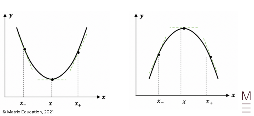
Because the first derivative indicated how the \(y\) value changed with respect to \(x\), the second derivative represents how the gradient \(\frac{dy}{dx}\) changes with respect to \(x\). This corresponds to the concept of concavity:

• If \(\frac{d^2 y}{dx^2}>0\), then the curve has an upward concavity (or is concave up)
• If \(\frac{d^2 y}{dx^2}<0\), then the curve has a downward concavity (or is concave down)

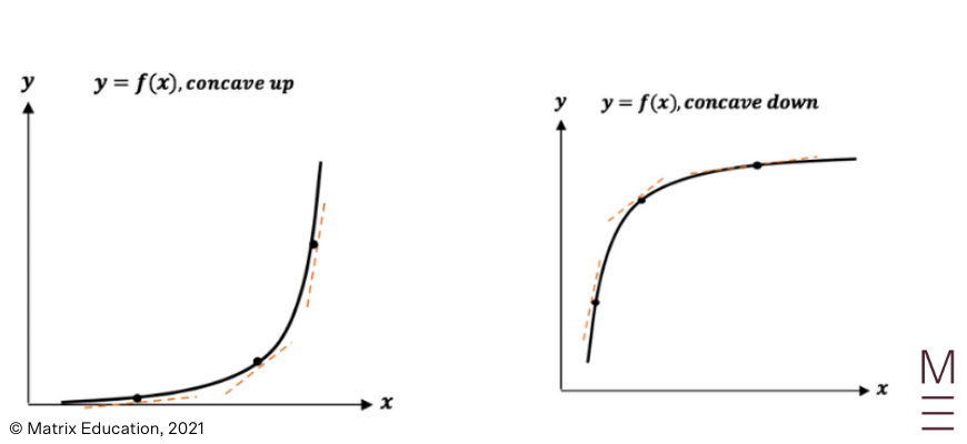
You can think of upward concavity as having a u-shaped while downward concavity has a \(n\)-shape. Note that a curve can be concave up and down at different points, just as how a curve can be increasing and decreasing at different points.

Point of Inflection

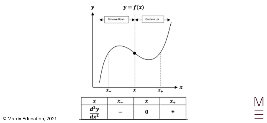
A point of inflection is a point where the concavity of the curve changes, and is defined to be when:

\(\frac{d^2 y}{dx^2}=0\) , and the sign of \(\frac{d^2 y}{dx^2}\) changes across the point.

For inflection points, students must remember to check if the sign of \(\frac{d^2 y}{dx^2}\) changes by creating a table of values or marks will be deducted in exams. Note that the inflection point is not exactly ‘flat’ like a stationary point, but rather the point where the concavity changes.

To identify points of inflection for a curve:

Example 1

Find the inflection points of the curve \(y=10-2x-x^2-x^3\).

Solution 1

Step 1:

Differentiate the function twice to find the second derivative

\begin{align*}
\frac{dy}{dx}&=-2-2x-3x^2  \\
\frac{d^2 y}{dx^2}& =-2-6x \\
\end{align*}

Step 2:

Let \(\frac{d^2 y}{dx^2}=0\)

\begin{align*}
-2-6x&=0 \\
-2&=6x \\
x&=-\frac{1}{3}\\
\end{align*}

Step 3:

Check if \(\frac{d^2 y}{dx^2}\) changes sign by creating a \(\frac{d^2 y}{dx^2}\) table

Setup the following table by:

• Placing the \(x\)-value of the inflection point in the middle of the table
• Choosing an \(x\)-value relatively close to the left and right of the inflection point (they do not have to be equally spaced away)
• Find the \(\frac{d^2 y}{dx^2}\) values at the chosen \(x\)-values (the centre value should be zero as that was assumed in the previous step)
• Check whether the sign changed at the inflection point

In this case, the sign did not change so it is not an inflection point at \(x=-\frac{1}{3}\) even though \(\frac{d^2 y}{dx^2 }=0\) at that point.

The Second Derivative Test for Stationary Points

Recall from Year 11 that a stationary point occurs when \(\frac{dy}{dx}=0\). The nature of the stationary point could be separated into minimum points, maximum points and stationary inflection points, and was previously determined by testing two points on the curve adjacent to the stationary point and on either side of it.

Alternatively, the second derivative can be used to test the nature of stationary points. By looking at the sign of \(\frac{d^2 y}{dx^2}\) at the stationary point (by subbing the relevant \(x\)-value into the second derivative), we can determine whether the graph is concave up or down and hence whether it is a maximum or minimum point.

• If \(\frac{d^2 y}{dx^2}>0\) at the stationary point, then it is concave up and hence must be a minimum point
• If \(\frac{d^2 y}{dx^2}<0\) at the stationary point, then it is concave down and hence must be a maximum point
• If \(\frac{d^2 y}{dx^2 }=0\) at the stationary point, then the point must be a horizontal point of inflection

Example 2

Determine the nature of the stationary points of the curve \(y=x^3+2x^2-7x+3\) by using the second derivative.

Solution 2

To find the stationary point, let \(\frac{dy}{dx}=0\):

To determine their nature, sub into \(\frac{d^2 y}{dx^2}\):

Curve Sketching Using Calculus

By applying the geometrical features of the first and second derivative, we can use this knowledge to aid us when sketching complex functions.

The following steps should be taken to identify the key information required in curve sketching:

Example 3

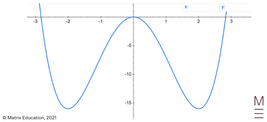
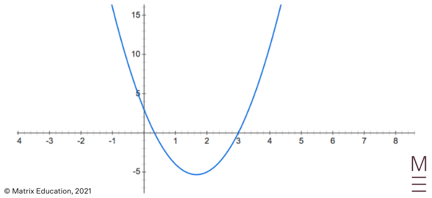
Sketch the curve of \(y=x^4-8x^2\), labelling stationary points and any points of inflexion.

Solution 3

Step 1:

Find the \(y\)-intercept

\begin{align*}
y \ int &=(0)^4-8(0)^2\\
&=0\\
\end{align*}

Step 2:

Consider the behaviour of \(y\) as \(x→±∞\).

when \(x→+∞,y→∞\)
when \(x→-∞,y→∞\)

Step 3:

Determine any stationary points and their nature by letting \(\frac{dy}{dx}=0\)

To determine the nature, evaluate \(\frac{d^2 y}{dx^2}\):

Step 4:

Determine any inflection points by letting \(\frac{d^2 y}{dx^2}=0\) and checking for changes to concavity

\begin{align*}
\frac{d^2 y}{dx^2}&=12x^2-16=0 \\
12x^2&=16\\
x^2&=\frac{4}{3}\\
∴x&=\frac{±2}{\sqrt{3}} \\
\end{align*}

∴inflection pt at \(\frac{2}{\sqrt3},-\frac{80}{9}\) and \(-\frac{2}{\sqrt{3}},-\frac{80}{9}\)

Step 5:

Sketch the curve, showing all essential features

Application of Maxima and Minima Problems

The process of identifying stationary points can be used to solve word problems where a certain value is to be maximised or minimised. To solve these problems:

Example 4

A fence is created on a farm using \(12\) metres of wire. It is bent into a rectangular shape against a barn such that the fourth (long side) of the fence is left open. Let the length of the rectangle be \(x\). Find the maximum area of the rectangle.

Solution 4

Step 1:

Create a formula for the quantity to be maximised or minimised

Drawing a diagram, a formula must be created for the area (which is to be maximised):

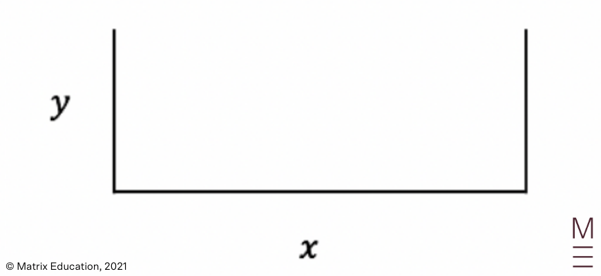
\(A=xy\),where \(y\) is the width of the rectangle

Step 2:

Simplify the formula to be in terms of only one independent variable, using other given information from the question

Recall that the total amount of wire used is \(12\) metres:

\begin{align*}
2y+x&=12 \\
y&=\frac{12-x}{2} \\
∴A&=\frac{x(12-x)}{2} \\
&=\frac{12x-x^2}{2} \\
\end{align*}

Step 3:

Solve for the stationary points by letting \(\frac{dA}{dx}=0\).

\begin{align*}
\frac{dA}{dx}&=\frac{12-2x}{2}=0 \\
12-2x&=0 \\
2x&=12 \\
x&=6 \\
\end{align*}

Step 4:

Check the nature of the stationary point to match what is required for the question

\begin{align*}
\frac{d^2 A}{dx^2}&=-\frac{2}{2}=-1<0 \\
\end{align*}

\begin{align*}
∴\text{A is maximised when }x&=6 \\
\end{align*}

Step 5:

Answer the question in words, including units

\begin{align*}
∴A_{max}&=\frac{12(6)-(6)^2}{2}=18 \\
\end{align*}

\begin{align*}
∴\text{the maximum area is }18m^2 \\
\end{align*}

Sketching the Gradient Function

Sketching the Gradient Function for a Given Function

Another common question in exams is sketching the graph of the derivative \(\frac{dy}{dx}\) given the graph of the curve \(y=f(x)\). These types of questions are difficult to master since they are purely graphical.

To sketch \(f'(x)\) from \(f(x)\):

Example 5

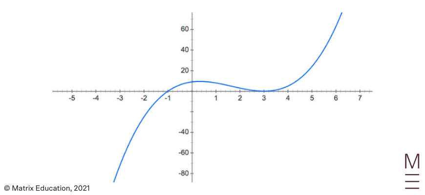
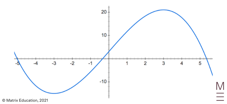
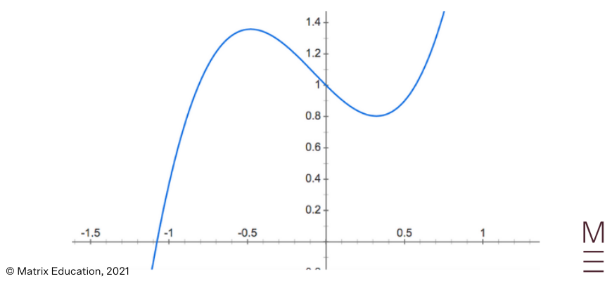
Sketch the derivative function of the following function:

Solution 5

Step 1:

Identify stationary points on the curve.

The stationary point of the given function is at \(x=0.2\) and \(x=3\). These will be the \(x\)-intercepts of the gradient function.

Step 2:

Identify where the curve is increasing.

The function is increasing at \(x<0.2\) and \(x>3\), so the gradient function will be positive at these values.

Step 3:

Identify where the curve is decreasing.

The function is increasing at \(0.2<x<3\), so the gradient function will be negative at these values.

Step 4:

Identify points of inflection on the curve The point of inflection of the curve is around \(x=1.8\), so the gradient function will have a stationary point (will be minimum as it is decreasing before and then increasing).

Sketching the Curve for a Given Gradient Function

Students may also be given a gradient function and expected to graph the curve based on this. To sketch \(f(x)\) from \(f'(x)\):

Example 6

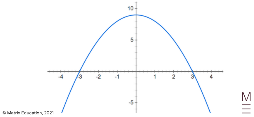
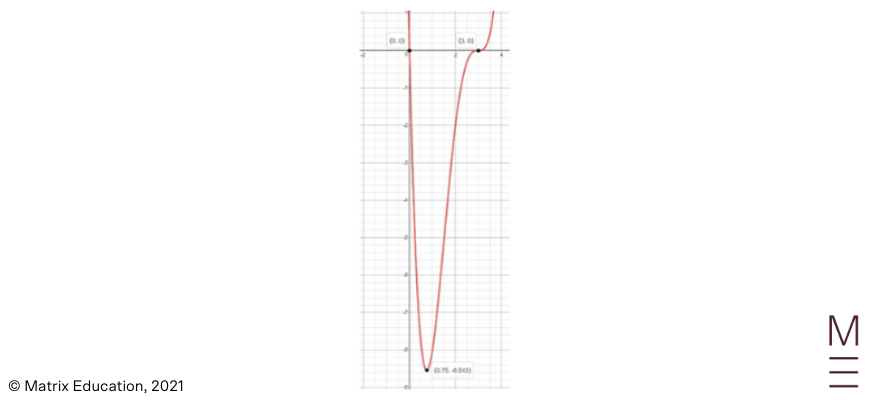
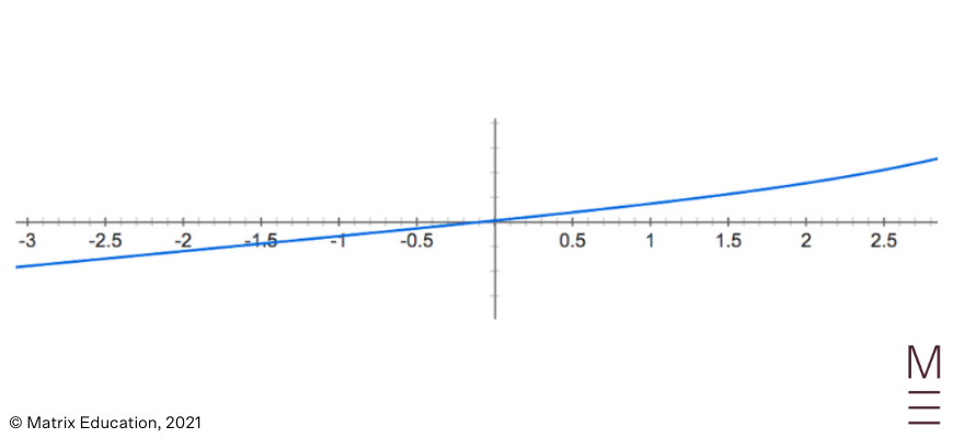
Sketch the function of the following gradient function:

Solution 6

Step 1:

Identify the \(x\)-intercepts of \(f'(x)\).

The \(x\)-intercepts are \(x=-3\) and \(x=3\). These will be the stationary points of \(f(x)\).

Step 2:

Determine the nature of the stationary points by examining the signs of \(f’ (x)\) directly before and after the stationary point.

For \(x=-3\), it is negative before and positive after so it will be a minimum point. For \(x=3\), it is positive before and negative after so it will be a maximum point.

Step 3:

Identify where the curve is increasing \((f’ (x)>0)\) and decreasing \((f’ (x)<0)\) to determine the shape of \(f(x)\).

The curve is positive at \(-3<x<3\) and negative at \(x<-3\) and \(x>3\).

Thus, the original function will look like:

Note that we do not know the \(y\)-intercept value and are not required to label it.

Graphs of Linear Motion

Review of Linear Motion

The concepts of differentiation can be applied to linear motion by considering the displacement, velocity and acceleration of a particle.

To recap, the displacement is the position of the particle from the origin. The instantaneous velocity measures how fast the particle is travelling at a particular instant, and is calculated as:

The acceleration is the instantaneous rate of change of velocity:

If \(a>0\), the velocity of the particle is increasing (i.e. going more positive or less negative)
If \(a<0\), the velocity of the particle is decreasing (i.e. going less positive or more negative)

Graphs of Linear Motions

Since the velocity and acceleration are the first and second derivatives of the displacement function, the geometrical properties can be obtained from the displacement-time graph. The velocity indicates the gradient while the acceleration represents the concavity of the curve.

In a velocity-time graph, the gradient of the curve represents the acceleration of the particle, since \(a=\frac{dv}{dt}\).

Example 7

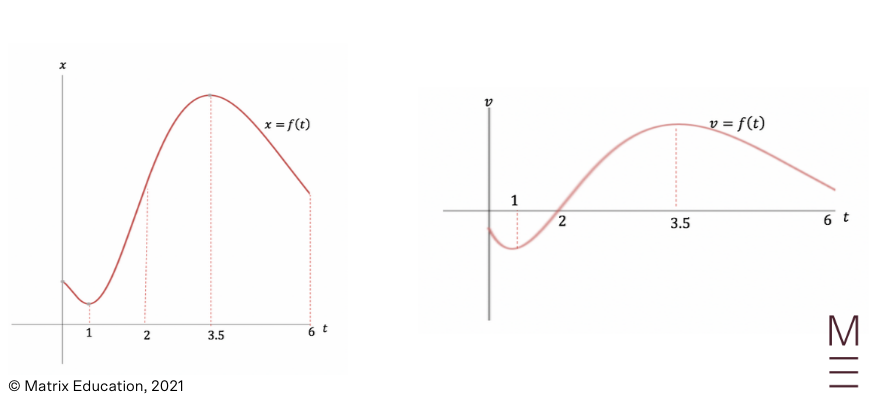
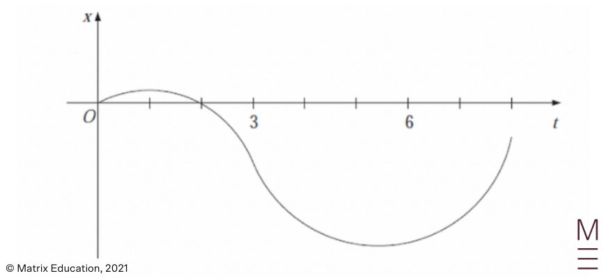
For the following displacement-time graph and velocity-time graph, at what times is there positive acceleration?

Solution 7

The first graph is a displacement-time graph, where the acceleration is represented by the concavity of the curve. As the graph is concave up at \(0≤t<2\), that is where there is positive acceleration.

The second graph is a velocity-time graph, where the acceleration is represented by the gradient of the curve. As the graph is increasing at \(1<t<3.5\), that is where there is positive acceleration.

Concept Check Questions

1. Consider the curve \(y=x(x-3)^3\).

a. Find the coordinates and nature of any stationary points of the curve.
b. Sketch the curve, indicating the coordinates of any intercepts and stationary points.

2. The cost, \(C\) (in thousands of dollars) for producing x (in hundreds) plates in a company is modelled by the equation:

\begin{align*}
C&=\frac{169}{2x+1}+2x, \ \text{where },0≤x≤20\\
\end{align*}

Determine the number of plates that must be produced to minimise the manufacturing costs and state the total cost.

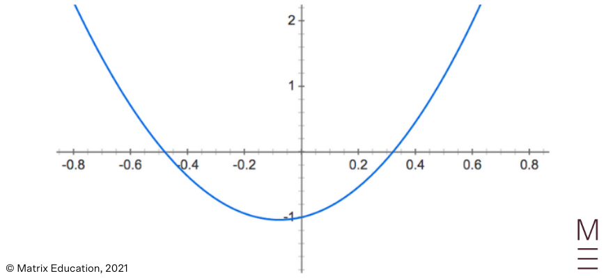
3. Draw the graph of the first and second derivative for the following curve:

4. The displacement-time graph of a particle is shown in the following diagram:

At what times is the velocity and acceleration equal to zero?

Concept Check Solutions

1.

a. Horizontal point of inflexion at \((3,0 )\), minimum point at \(\left(\frac{3}{4},-\frac{2187}{256}\right)\)
b.

2. The cost is minimised when \(600\) parts are plates are manufactured and the total cost will be \(\$ 25 \ 000\).

3. First derivative:

Second derivative:

4. \(\text{Velocity}:1s,5.75s,\text{ Acceleration}:3s\)

Worried your curve sketching is…. well, sketchy?

Get detailed feedback and improve your confidence with graphs and sketching. Revise all Maths Adv core topics with our HSC experts and practise your exam skills. Learn more about our Year 12 Maths Adv Course.