Part 2: Integration | Beginner’s Guide Year 12 Maths

Unsure about integration for Year 12 Maths Advanced? In this article, we’re going to give you a detailed rundown of Year 12 Integration so you have the right fundamentals for your HSC.

In this article we’ll discuss:

• The NESA syllabus outcomes
• Assumed knowledge
• The Primitive Function
• Definite Integrals
• Area Under a Curve
• Area Between Two Curves
• Trapezoidal Rule
• Concept Check Questions
• Concept Check Solutions

Need to test your integration skills?

Download our free worksheet and see what your strengths and weaknesses are.

Year 12 Advanced Mathematics: Integration

Integration is an important concept that will be explored in this blog to evaluate areas, and this will provide the fundamentals behind determining the volume of solids later in the year.

Now that you know differentiation, it is important to understand the opposite process, integration. It can be applied to evaluate the area under a given curve and will be used extensively across the Year 12 course.

This resource will provide you with an outline of the best techniques to use when approaching integration problems.

NESA Syllabus outcomes

C4.1: The anti-derivative

Students:

• Define anti-differentiation as the reverse of differentiation and use the notation  for anti-derivatives or indefinite integrals
• Establish and use the formula \( \int x^{n} \ dx = \frac{1}{n+1} x^{n+1} + c, \ for \ n \ \neq 1 \)
• Determine indefinite integrals of the form \( \int f(ax +b) \ dx \)
• Determine \( f(x) \) given \( f'(x) \) and \( f(a) = b \) an initial condition  in a range of practical and abstract applications including coordinate geometry, business and science

C4.2: Areas and the definite integral

Students:

• Know that ‘the area under a curve’ refers to the area between a function and the ?-axis, bounded by two values of the independent variable and interpret the area under a curve in a variety of contexts
• Use the notation of the definite integral \( \int_{a}^{b} f(x) \ dx \) for the area under the curve \( y = f(x) \) from \( x = a \) to \( x = b \) if \( f(x) \geq 0 \)
• Use the Trapezoidal rule to estimate areas under curves
  • Use geometric arguments (rather than substitution into a given formula) to approximate a definite integral of the form\( \int_{a}^{b} f(x) \ dx \), where \( f(x) \geq 0 \), on the interval \( a \leq x \leq b\), by dividing the area into a given number of trapezia with equal widths
  • Demonstrate understanding of the formula:
    

    \( \int_{a}^{b} f(x) \ dx \approx \frac{b – a}{2n} \) \( [f(a) + f(b) + 2 \{ f(x_{1}) + … + f(x_{n-1}) \}] \)

    where \( a = x_0 \) and \( b = x_n \) and the values of \( x_{0}, x_{1}, … , x_{n} \) are found by dividing the interval into \( n \) equal sub-intervals

• Understand the relationship of position to signed areas, namely that the signed area above the horizontal axis is positive and the signed area below the horizontal axis is negative
• Calculate the area under a curve
• Calculate areas between curves determined by any functions within the scope of this syllabus
• Integrate functions and find indefinite or definite integrals and apply this technique to solving practical problems

Assumed knowledge

You should be comfortable with practical applications of calculus, including:

• Interpreting the relationship between the first and second derivatives and the original function
• Knowledge of the theorems for differentiation, including the chain, product and quotient rules

1. The Primitive Function

Introducing the Primitive Function

Throughout the past year, students would have encountered the process of differentiation which involved calculating the derivative of functions.

Now, we introduce the concept of integration, which essentially reverses the process of differentiation.

For example, if you are given the gradient function of a curve, you can find the equation of the original curve by using the process of anti-differentiation, or “taking the primitive of a function”.

The primitive of function \( f(x) \) is denoted as \( F(x) \), or in other words:

 \( F'(x) = f(x) \)

General Rules for Finding the Primitive

To find the primitive of a function, the following general rules can be used:

• Primitive of \( x^{n} \):

• Primitive of a constant \( k \):

• Primitive of a constant \( kg(x) \):

• Primitive of a sum or difference of functions:

One issue that arises when finding primitives is that when you differentiate a function, constants are removed. Thus, there may be more than one possible primitive for a given function.

To account for all the positive primitives a function may have, we add a \( +C \) at the end of the primitive to represent “plus a constant”.

Always remember to include the constant when finding the general primitive of a function or marks will be deducted.

Example 1

Find the primitive of \( f(x) = 3x^{2} – x^{-2} \).

Solution 1

Using the general rules for finding the primitive:

$$
F(x) = 3 \times \frac{x^{3}}{3} – \frac{x^{-1}}{-1} + C \\
= x^{3} – x^{-1} + C
$$

Example 2

Find the primitive of \( f(x) = \frac{\sqrt{x}}{3} – \frac{2}{5x^{2}} + 3 \).

Solution 2

By first rewriting and then applying the rule:

\begin{align}
f(x) &=\frac{x^{\frac{1}{2}}}{3} – \frac{2}{5}x^{-5} + 3 \\
F(x) &= \frac{\frac{x^{3}}{2}}{3 \times \frac{3}{2}} – \frac{2}{5} \times \frac{x^{-4}}{-4} + 3x + c \\
&= \frac{x^{3}}{9} + \frac{x^{-4}}{10} + 3{x} + C
\end{align}

Finding the Particular Equation of a Primitive Function

Students may be required to evaluate the equation of a function, which would require the specific constant \( (C) \) of that equation to be found.

If we are asked to find the particular primitive function, given it passes through the point \( (x_{1}, y_{1})\), the following process should be followed:

Example 3

Let \( f'(x) = 6x^{2} – 2 \). Find the equation of the curve \( f(x) \) given that it passes through the origin.

Solution 3

Step 1: Find the primitive of the gradient function, including the \( +C \)

\begin{align}
F(x) &= \frac{6x^{3}}{3} – 2x + C \\
&= 2x^{3} -2x + C
\end{align}

Step 2: Substitute in the given point \( (x_{1}, y_{1})\) to find the particular value of \( C \).

\begin{align}
0 &= 2(0)^{3} – 2(0) + C \\
∴ C &= 0
\end{align}

Step 3: Rewrite the equation with the newly found value of \( C \)

\begin{align}
F(x) = 2x^{3} – 2x
\end{align}

The Reverse Chain Rule

Rearranging the chain rule learnt using differentiation, the reverse chain rule is given by:

Example 4

Find the primitive of \( (2x – 5)^{6} \), using the reverse chain rule.

Solution 4

Using the reverse chain rule:

\begin{align}
F(x) &= \frac{(2x – 1)^{6}}{6 \times 2} + C \\
&= \frac{(2x -1)^{6}}{12} + C
\end{align}

Integral Notation

Another notation for finding the primitive of a function is the integral sign \( \int \).

It is called the ‘Indefinite Integral’ and will be very useful later in this blog when we evaluate the area under curves.

\begin{align}
\int f(x) \ dx = F(x) + C \\
\end{align}

This integral notation is commonly used when finding primitives and all the rules previously explained still apply.

2. Definite Integrals

In certain situations, it may be required to evaluate integrals between two specific values,  \( x = a \) and \( x=b \). This is called a ‘Definite Integral’ and is denoted by:

\begin{align}
\int_{a}^{b} f(x) \ dx = [ F(x)]_{a}^{b} = F(b) \ – \ F(a)
\end{align}

To evaluate definite integrals:

Example 5

Find \( \int_{1}^{5} 9x^{2} \ dx \).

Solution 5

Step 1: Find the primitive of \( f(x) \) like before, but don’t include the constant \( C \). Instead, place square brackets around the function and include the limits.

\begin{align}
\int_{1}^{5} 9x^{2} \ dx &= \Big[ \frac{9x^{3}}{3} \Big]_{1}^{5} \\
& = [3x^3]_{1}^{5}
\end{align}

Step 2: Substitute the limits \( F(x) \) into subtracting the lower limit by the upper limit.

\begin{align}
\int_{1}^{5} 9x^{2} \ dx = 3(5)^{3} – 3(1)^{3}
\end{align}

Step 3: Simplify the value of the definite integral

\begin{align}
\int_{1}^{5} 9x^{2} \ dx = 375 – 3 = 372
\end{align}

Example 6

Find \( \int_{0}^{1} (1 + 10x – 3x^{2}) dx \)

Solution 6

Step 1: Find the primitive of \( f(x) \) like before, but don’t include the constant \( C \). Instead, place square brackets around the function and include the limits.

\begin{align}
\int_{0}^{1} (1 + 10x – 3x^{2}) dx = [x + 5x^{2} – x^{3} ]_{0}^{1}
\end{align}

Step 2: Substitute the limits into subtracting the lower limit by the upper limit

Step 3: Simplify the value of the definite integral

\begin{align}
\int_{0}^{1} (1 + 10x – 3x^{2}) \ dx = 5 – 0 = 5
\end{align}

3. Area Under the Curve

Regions above the x-axis

Integration can be used to also evaluate the area under a given function.

The area of the shaded region bounded by the curve \( y = f(x) \), the \( x \)-axis and the lines \( x = a \) and  can \( x = b \) be calculated by

\begin{align}
A = \int_{a}^{b} f(x) dx
\end{align}

Example 7

Calculate the area of the region bounded by the curve \( y = x^{2} + 9 \), the \( x \)-axis, and the lines \( x = 1 \) and \( x = 3 \).

Solution 7

Step 1: Draw a diagram to indicate the required region above the \( x \)-axis.

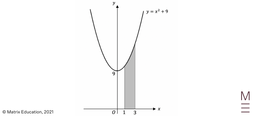
Step 2: Use the equation to \( A = \int_{a}^{b} f(x) \) write the area in terms of a definite integral

\begin{align}
A &= \int_{1}^{3} x^{3} + 9 \ dx \\
&= \left[ \frac{x^{3}}{3} + 9{x} \right]_{1}^{3}
\end{align}

Step 3: Integrate and simplify, ensuring that your answer includes

\begin{align}
A &= \left[ \frac{3^{3}}{3} + 9(3) \right] – [\frac{1^{3}}{3} + 9(1) \big] \\
&= 36 – \frac{28}{3} \\
&= \frac{80}{3} \ units^{2}
\end{align}

Regions below the \(x\)-axis

One thing to notice is that the definite integral can potentially give a value that is negative. This corresponds to regions where the curve is actually below the x-axis, as this will mean that the shaded area is actually below the \(x\)-axis as well.

However, areas cannot be negative so students must take extra care in these situations. Some questions will have an area of region that is sometimes above and sometimes below the x-axis. All pieces of these areas should be treated as positive, so it may be required to separate the area into different integrals with absolute value signs.

Example 8

Calculate the area of the region bounded by the curve \( y=x^2-1\), the \(x\)– axis, and the lines \(x=0\) and \(x=1\).

Solution 8

Step 1: Draw a diagram to indicate the required regions.

Step 2: Determine where the region is above and below the \(x\)-axis.

Based on the diagram, the region is below the \(x\)-axis between \(x=0\) and \(x=1\). There is no need to separate the area into separate integrals since it is all below the \(x\)-axis.

Step 3: Write the area in terms of the separated integrals.

\begin{align*}
A &= \left| \int_0^1 x^2 – 1 dx \right| \\
\end{align*}

Step 4: Integrate and simplify, ensuring that your answer includes \(\text{units}^2\).

\begin{align*}
A & = \left|\left[\frac{x^3}{3} – x\right]^1_0 \right| \\
&=\left|\left(\frac{1^3}{3}-1\right) – \left(\frac{0^3}{3} – 0\right) \right| \\
& = \left| -\frac{2}{3}\right| \\
&= \frac{2}{3} \text{units}^2 \\
\end{align*}

4. Area Between Two Curves

To evaluate the area between two curves in a specific interval, you can imagine first calculating the area under the top graph and then subtracting it with the area under the bottom graph for the same interval. Hence, the area of the region bounded by two curves in the domain \(a≤x≤b\) is:

\begin{align*}
A=\int^b_a \text{Top} \ – \ \text{Bottom} \ dx \\
\end{align*}

Example 9

Find the area of the following shaded region:

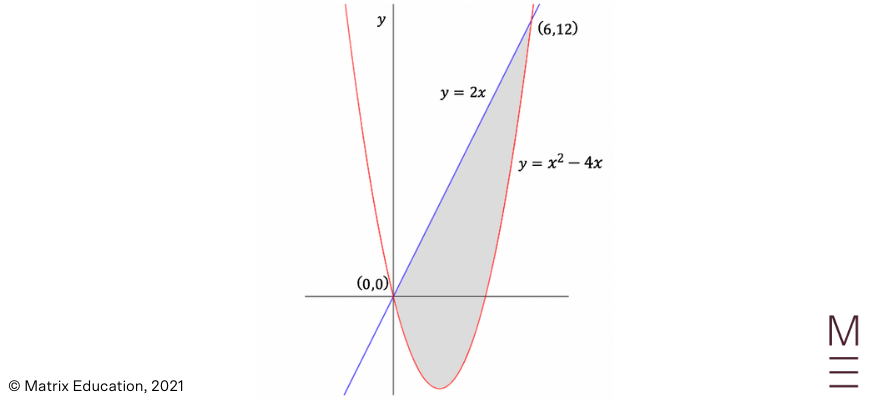
Solution 9

Step 1: Determine the limits of integration by finding the points of intersection of the graphs.

The point of intersection of the graphs is (\(0,0\)) and (\(6,12\)) based on the given graph.

Step 2: Use the formula \(A=\int^b_a \text{Top} – \text{Bottom} \ dx\) to express the area as a definite integral.

\begin{align*}
A & = \int^6_0[2x-(x^2 – 4x)] dx \\
& = \int^6_0 6x-x^2 \ dx \\
\end{align*}

Step 3: Integrate and simplify, ensuring that your answer includes \(\text{units}^2\).

\begin{align*}
A&=\left[3x^2-\frac{x^3}{3}\right]^6_0 \\
&=\left[3(6)^2 – \frac{(6)^3}{3}\right]-\left[3(0)^2 – \frac{(0)^3}{3}\right] \\
&=36-0 \\
&=36 \ \text{units}^2 \\
\end{align*}

5. Trapezoidal Rule

In some cases where we encounter a function that we do not know how to integrate, we can still approximate the area bounded by a curve \(y=f(x)\), the \(x\)-axis and the lines \(x=a\) and \(x=b\) using the Trapezoidal Rule.

This rule approximates the area by dividing the interval into \(n\) subintervals and summing trapeziums under the curve. The Trapezoidal Rule is given by:

As the number of subintervals \(n\) increases, the approximation usually becomes more accurate.

Example 10

The values of a function \(f(x)\) in the domain \(0≤x≤2\) are given in the table below:

Use the Trapezoidal Rule and the five function values to approximate \(\int^2_0 f(x)dx\)

Solution 10

Step 1: Divide the interval \(a≤x≤b\) into \(n\) equal subintervals.

In this question, \(n=4\) as there are \(4\) sub-intervals (and \(5\) function values).

Step 2: Draw a table of values for the \((n+1)\) function values and substitute into the function to calculate values of \(y\).

In this example, the table is are already provided within the question. Note that during exams, the question might already provide the values rather than state a function to approximate.

Step 3: Substitute into the formula by summing the first and last values and adding twice the middle values.

Concept check questions

1. Evaluate:

a. \(\int^3_{-2}(x^2-1)dx\)
b. \(\int (5-3x)^5 -5\sqrt{x} \ dx \)

2. Evaluate the area of the region bounded by the curve \(y=x^3-4x\) and the \(x\)-axis in the domain \(-1≤x≤2\).

3. Find the area of the region bounded by the parabolas \(y = x^2\) and \(y=2x-x^2\).

4. Use the trapezoidal rule and \(5\) subintervals to approximate \(\int^1_{1.5} 2^{x+1}dx\) correct to \(3\) decimal places.

Concept check solutions

1.

a. \(\frac{20}{3}\)
b. \(\frac{(5-3x)^6}{-18} – \frac{10x^{\frac{3}{2}}}{3} + C\)

2. \( \frac{23}{4} \text{Units}^2\)

3. \( \frac{1}{3} \text{Units}^2\)

4. \(4.798 \ (3 dp)\)

Boost your marks and your rankings before your HSC

It’s your last chance to boost your HSC marks. Revise all Maths Adv core topics with our HSC experts and practise your exam skills with our mock exam. Learn more about our HSC Prep Course.