Module 5: Advanced Mechanics

In this article, we’re going to help you get on top of Advanced Mechanics. We’ll give you an overview of the Module before giving you in-depth explanations of the three main areas of study.

Advance your understanding of Advanced Mechanics

Download your FREE foldable Physics Cheatsheet

Get the competitive edge for your next Physics assessment!

Download now

Download your FREE foldable Physics Cheatsheet

Fill out your details below to get this resource emailed to you.

"*" indicates required fields

First Name*

Last Name*

Email*

Postcode*

Grade in 2025*

Grade in 2025123456789101112

Hidden

Resource (DO NOT DELETE OR CHANGE)

By submitting this form, you agree to receive promotional messages from Matrix about its products and services. You can unsubscribe at any time by clicking on the link at the bottom of our emails.

What is Advanced Mechanics?

Advanced Mechanics can be separated (roughly) into three areas:

1. Projectile Motion
2. Circular Motion
3. Gravitational Motion

Let’s have a closer look.

Projectile motion

Projectile motion in Advanced Mechanics is an extension of the one-dimensional projectile motion you have studied in Year 11 in two-dimensional problems.  As such, we’re first going to start by revisiting and modifying existing Year 11 concepts:

The Variables of Motion

In Year 11 you used the variables \(s\), \(v\),  and \(a\) to represent the displacement, velocity and acceleration of an object.

In extending this to two dimensions, we now need to use two different sets of variables. The ‘\(x\)’ axis variables which typically refers to horizontal motion. And, the ‘\(y\)’ axis variables, which typically refers to vertical motion:

• \(x\) or \(s_x\) – displacement in the \(x\) axis
• \(y\) or \(s_y\) – displacement in the \(y\) axis
• \(u_x\)  and \(v_x\) – the initial velocity in the \(x\) axis, and the final velocity in the \(x\) axis
• \(u_y\)  and \(v_y\) – the initial velocity in the \(y\) axis, and the final velocity in the \(y\) axis
• \(a_x\) – the acceleration in the \(x\)-axis
• \(a_y\) – the acceleration in the \(y\)-axis
• \(t\) – the time of flight

An important thing to keep in mind is that the \(x\) and \(y\) axes are independent of one another – the position, velocity and acceleration of an object in the \(x\) direction have no impact on the position, velocity and acceleration of an object in the \(y\) direction, and vice versa.

In fact, the only thing these two dimensions have in common is time. Whenever the motion is stopped in one dimension (for example, a ball hitting the ground after falling in the \(y\) direction), the motion in the other direction also stops. In other words, there is no such thing as \(t_x\) or \(t_y\): the motion in each axis shares a common time \(t\).

The Equations of Motion

A key skill you developed in Year 11 was the use of the equations of motion that related the variables \(s\), \(u\), \(v\), \(a\) and \(t\):

• \(v=u+at\)
• \(s=ut+ \frac{1}{2} at^2\)
• \(v^2=u^2+2as\)

You’ll recall that these equations were valid only for constant acceleration (and zero is a constant, too!)

In order to extend these equations to 2-dimensions, we are going to make use of the following assumption: the acceleration in one of the dimensions is zero.

The simplest example of this is a projectile motion under gravity: since gravity only acts in the vertical (\(y\)) direction. So, we can set the acceleration in the horizontal (\(x\)) direction to be zero. Setting \(a_x=0\) results in rather simple horizontal equations of motion:

• \(v_x=u_x\)
• \(x=u_x t\)

Of course, the equations of motion in the vertical direction are a little more complex:

• \(v_y=u_yt\)
• \(y=u_y t+ \frac{1}{2} a_yt^2\)
• \(v_y^2=u_y^2+2a_y y\)

If the problem is one under gravity, you will be expected to know that \(a_y=g=-9.8 ms^{-2}\) (since we generally assume up is positive \(y\) direction).

Vector Decomposition

Importantly, you may not always receive information in \(x\) and \(y\) co-ordinates.

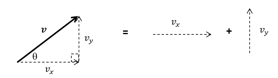
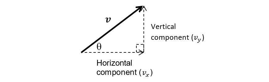
If you have been given a vector with a magnitude and direction (i.e. an angle, \(θ\)), recall that you can extract the \(x\) and \(y\) components via trigonometry; in the example above, you can use:

• \(v_x=v \ cos(θ)\)
• \(v_y=v \ sin⁡(θ)\)

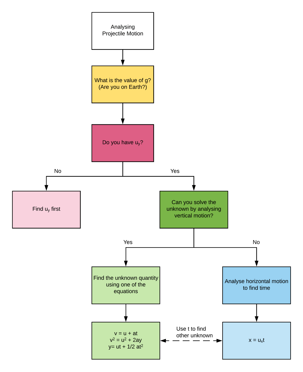
Solving These Equations

The flowchart below outlines a general method for solving 2D projectile motion equations. (This may not apply to all situations so first check what is being asked in the question!)

Send your Physics marks into orbit!

Give you marks the last-minute push they need. The Matrix+ Physics HSC prep course provides you with one-to-one feedback and expert help. Learn more.

Circular Motion

Similarly to projectile motion, the circular motion topic expands from the Uniform Circular Motion (UCM) topic of Year 11.

In Year 12, you learn to consider the force(s) that cause an object to undergo UCM, the energy of an object undergoing UCM, and an object travelling a circular path at varying speeds – non-uniform circular motion!

Uniform Circular Motion Characteristics

Form Year 11, we know the characteristics of uniform circular motion are:

• The object moves at a constant speed (uniform)
• The object moves in a perfect circle (circular)
• The object’s velocity is constantly changing.
  The magnitude remains the same, but the direction varies such that the object maintains its circular path.

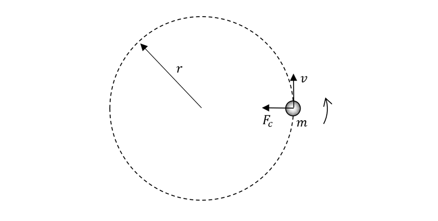
In this module, we introduce the concept of centripetal force as the force that causes the object to continuously change direction.

Causing Uniform Circular Motion

From Newton’s second law (\(F_{net}=ma\)), we know that any acceleration is resultant from a net force. An object undergoing uniform circular motion experiences a change in velocity (due to the change of direction of its motion) and therefore is undergoing acceleration. Since all acceleration results from a net force, we can presume that a force is causing this object to undergo uniform circular motion. This force is known as centripetal force.

Centripetal force always acts towards the centre of rotation: it is perpendicular to the velocity of the object. A perpendicular force means that centripetal force only changes the direction of velocity, not its magnitude. The case of a non-perpendicular force will be examined later in this section.

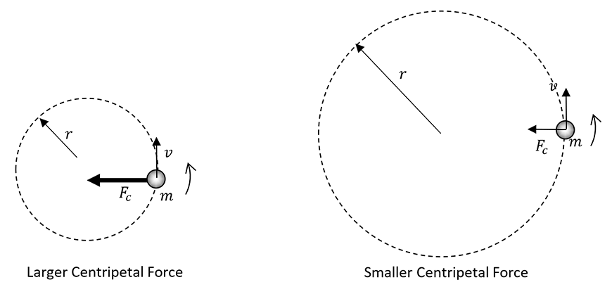
Centripetal force is given by the equation \(F_c=\frac{(mv^2)}{r}\), where:

• \(F_c\) is the centripetal force
• \(m\) is the mass of the object
• \(v\) is the speed of the object
• \(r\) is the radius of the circle the object is travelling in.

You can qualitatively confirm this relationship by spinning a heavy object on a string: the string (via your hand) provides the centripetal force that keeps the object moving in a circle.

• If you increase the speed of rotation, you require more force to keep the object moving in a circle!
• Likewise, if you decrease the radius of the circle (by using a shorter string), you will find that the object requires more force to maintain a circular path.

Other Circular Motion Relations

There are a few other relationships in uniform circular motion that are necessary to understand:

Centripetal Acceleration

By combining Newton’s Second Law with our expression for Centripetal Force (i.e. dividing \(\frac{mv^2}{r}\) by \(m\)), we arrive at the formula for centripetal acceleration: \(a_c=\frac{v^2}{r}\). This formula is used when mass is not given, or not important to the situation.

Period, Velocity, Radius

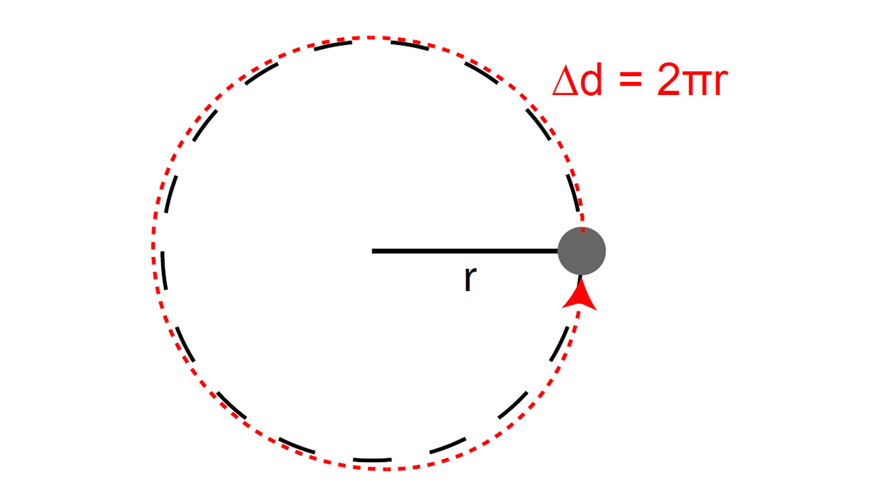
In UCM situations where the velocity is not given, it can be derived by recalling the simple equation \(v=\frac{\Delta d}{t}\).

For an object undergoing UCM, the distance travelled in one revolution (trip around the circle) is the circumference; \(\Delta d=2πr\).

The time taken for one revolution is known as the Period, \(T\).

From this, we can derive the linear velocity of an object undergoing UCM as:

\(v=\frac{2πr}{\Delta t}\)

Angular Velocity

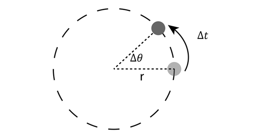
Another way of thinking about the velocity of an object undergoing UCM is by considering the angular change. The angular velocity ω (in radians per second) of an object is the number of radians it rotates every second.

This can be calculated by determining the total change-in-angle (\(Δθ\)) the object undergoes in a certain amount of time (\(Δt\));

\(ω=\frac{Δθ}{Δt}\)

A special case is when you already know the period (\(T\)) of rotation – by definition, this is the time it takes for the object to rotate \(2π\) radians! If you know this value, you can determine the angular velocity using:

\(ω=\frac{2π}{T}\)

Can you see the similarities between this equation and our equation for linear velocity? From this, we can infer that angular velocity and linear velocity are related via the following:

\(v=ω \ r\)

Where \(v\) is in metres per second, \(ω\) is in radians per second, and \(r\) is the radius of the circular path.

Energy in UCM

If an object is undergoing uniform circular motion, the speed is constant, and therefore the kinetic energy is also constant. Unless this object is undergoing a change of potential energy (unlikely if it’s still uniform circular motion), the kinetic energy and potential energy are constant.

If the energy is constant, we know that the work done on the rotating object should be zero:

\(W=ΔE=0\)

By recalling our work-done equation (\(W=Fs \cos(θ)\)), we can see that work will be zero if \(θ\) – the angle between the force vector and direction of motion – is \(90\) degrees. We have already said this is the case for the centripetal force that causes UCM, and, therefore, we can confidently say that no work is done on an object undergoing uniform circular motion.

Torque and Non-Uniform Circular Motion

Torque is a measure of the turning-capacity of an applied force. For a Force \(F\) applied at some point \(r\) away from the centre-of-rotation, the torque applied will be:

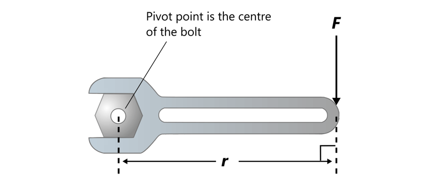
\(τ=rF \sin(θ)\)

Where \(θ\) is the angle between the force vector and the line joining the centre-of-rotation and the point where the force is applied (the vector \(r\)).

Just like how a net force causes changes in linear motion of objects, a net torque causes a change in rotational motion of the object.

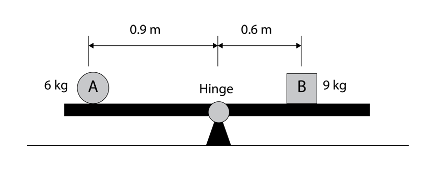
For an object to remain at a constant rotation (including being stationary), the net torque must be zero – not the net force!

For example, this see-saw has different masses on each arm but the torque on each side is equal: the see-saw is balanced and does not rotate.

An applied torque on an object moving in a circle will cause a change in speed and/or a deviation in path depending on the details of the scenario. If a non-zero net torque is applied to an object, it cannot undergo uniform circular motion.

Gravitational Motion

You have seen problems involving motion under uniform gravity – where the force on the object is constant in both direction and magnitude.

In this section, we will consider objects undergoing motion where the force of gravity is not constant in either magnitude, direction or both. These scenarios involve the motions of planets and satellites: the only objects that move through large enough distances to experience changing gravitational force.

Newton’s Law of Universal Gravitation

In addition to his three laws of motion, Isaac Newton also developed the law of universal gravitation, which calculates the gravitational force of attraction between two objects. This is given as:

\(F=\frac{GMm}{r^2}\)

Where:

• \(F\) is the force between the objects (newtons)
• \(r\) is the separation between the centres of the objects (meters)
• \(M\) the mass of one object (usually the larger one, kilograms)
• \(m\) is the mass of the second object (usually the smaller one, kilograms)
• \(G\) is the gravitational constant \(= 6.674×10^{-11}   \frac{{N \ m}^2}{kg^2}\)

Note that, the force is the same on each object (but the acceleration from this force will not be).

From this formula, we can derive an expression for \(g\), the acceleration a (smaller) object experiences by being in the gravitational field of a larger one. By considering the force on the smaller mass \(m\) using Newton’s Second Law:

\(F=\frac{GMm}{r^2} =ma→a=\frac{GM}{r^2} =g\)

From this expression, we can predict the change in the strength of a gravitational field if we were further away from the centre of the Earth (larger \(r\), so smaller \(g\)), or if we moved to a more massive planet (larger \(M\), so larger \(g\)).

Circular Satellite Orbits

Newton’s Law of Universal Gravitation allows us to easily understand circular orbits of satellites. A satellite orbiting a planet in a circle is undergoing uniform circular motion, and so requires a centripetal force – this force is provided by the gravitational force between the planet and the satellite.

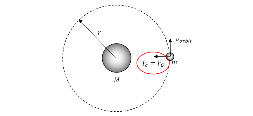
This allows us to combine the gravitational force and centripetal force expressions and arrive at an equation for the orbital speed of a satellite.

\(F_c=\frac{mv_{orbit}^{2}}{r}=F_G=\frac{GMm}{r^2} →v_{orbit}=\sqrt{\frac{GM}{r}}\)

Aside from this interesting relation (notice how the satellite’s orbital speed doesn’t depend on its own mass!), analysis of circular orbits is identical to other uniform circular motion problems.

Kepler’s Laws

Prior to Newton, Johannes Kepler observed the motions of the planets and derived Kepler’s Three Laws of Planetary Motion. While these laws described the motion of the planets correctly, they did not explain the motion (this was done by Newton’s laws later).

Kepler’s first law – the Law of Ellipses – states that the orbit of every satellite is elliptical, with the central body (such as the Sun) at one of the foci of the ellipse.

Elliptical motion is harder to analyse than uniform circular motion, and as such you aren’t required to do any quantitative analysis on elliptical orbits, as you have done on circular orbits.

Kepler’s second law is the Law of Areas, which states that each planet moves so that the radius vector (the line joining the planet and central body) sweeps out equal areas in equal times. This is shown in the diagram below: both of the shaded areas are the same, but one has a short radius vector and large angle-of-sweep, and one has a large radius vector and small angle-of-sweep.

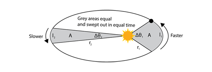
The consequence of Kepler’s second law is that objects in elliptical orbits travel faster when they are closer to the central body.

Kepler’s third law is referred to as the Law of Periods, and it states that for any object(s) orbiting the same central body, \(\frac{r^3}{T^2}\)  is constant (where \(r\) is the average radius of the orbit, and \(T\) is the period of the orbit). Using Newton’s Law of Universal Gravitation, the value of this constant can be derived, yielding the more common equation:

\(\frac{r^3}{T^2} =\frac{GM}{4π^2}\)

Note that, the equation above is only valid when using \(SI\) units for all quantities. If non-\(SI\) units are used for \(r\) and \(T\), \(\frac{r^3}{T^2}\) will still be a constant, but the value of this constant will not be \(\frac{GM}{4pi^2}\).

Energy and Escape Velocity

In Year 11, you learned that the gravitational potential energy of an object of mass ‘\(m\)’ was given by \(U=mgh\), where \(g\) was the acceleration due to gravity and h was the height above some reference point.

To extend this equation to cover non-uniform gravity, we make the following changes;

• Substitute in our expression for \(g=\frac{GM}{r^2}\)
• Decide that \(h = 0\) at the centre of the central body, meaning \(h=r\)

Using these, we arrive at the equation for gravitational potential energy:

\(U= – \frac{GMm}{r}\)

Notice the negative sign out the front – this is by convention: in broader physics we consider potential energies to be negative. (The potential energy still increases as r increases.)

The Kinetic energy of a satellite can be derived from our normal kinetic energy expression, \(K=\frac{1}{2} mv_{orb}^{2}\) and the expression for orbital velocity: \(v_{orb}= \sqrt{\frac{GM}{r}}\):

\(K=\frac{1}{2}\frac{GMm}{r}\)

We can combine these two expressions to get the total energy of an orbiting satellite:

\(U+K= – \frac{GMm}{2r}\)

Where \(r\) in this expression is the average orbital radius of the satellite.

From this, we can make an interesting conclusion: whenever the average radius of an orbit increases, so does the energy of the satellite. If a satellite had to move to a higher altitude orbit it’s energy would increase. Hence, work would be required to be done on satellite.

The final concept to understand is escape velocity – the minimum velocity you must have at a given point in a gravitational field to escape the gravitational field forever.

We can break this down into a couple of energy requirements:

• To leave the gravitational field, we need to get to \(r=∞\)
  • This corresponds to a potential energy of \(U= \frac{-GMm}{∞}=0\)
  • We recall from Year 11 that gravitational motion follows the conservation of mechanical energy: \(ΔK= -ΔU\) – the change in potential energy is equal in magnitude to the change in kinetic energy.
• If we had the ‘minimum velocity’ needed to achieve this, our kinetic energy would be zero just as we reached \(r=∞\).
  • To make both \(U\) and \(K=0\) at this endpoint, they must have the same value (opposite sign) to begin with, as they will be changing by the same amount throughout the journey.
• The conclusion we can make is – in order to have escape velocity, our kinetic energy must be equal in magnitude (but opposite in sign) to the current potential energy:

\(K=-U→  \frac{1}{2} mv_{esc^2}=\frac{GMm}{r}\)

This gives the following expression for escape velocity: \(v_{esc}= \sqrt{\frac{2GM}{r}}\)