Welcome to Matrix Education
To ensure we are showing you the most relevant content, please select your location below.
Select a year to see courses
Select a year to see available courses
Struggling to get the ball rolling with your Physics marks? In this Guide, we’ll walk you through Module 1 Kinematics for year 11 Physics so your marks get the right kind of momentum!
Get your Physics marks on the move
Get the competitive edge for your next Physics assessment! 
Download your FREE foldable Physics Cheatsheet
Before we study the physics behind how objects behave and interact, we need to establish a precise system of language and mathematics to describe our observations. In Year 11, we will be using more technical language compared to previous years; some words which have a broad meaning in everyday life (such as ‘energy’ and ‘work’) have a specific meaning in the context of physics, and so we must ensure we all agree on their definitions.
Kinematics is the description and analysis of the motion of objects without studying the cause of the motion.
We will start by introducing the concept of vector quantities. From there, we will apply our knowledge to describing one-dimensional motion, followed by expanding to motion on a plane.
In physics, we deal with a variety of quantities such as mass, distance, energy, etc.
Physical quantities can be classified into two main categories:
In kinematics, the vectors of interest are:
All of these quantities have a magnitude and direction, and they are mathematically related to each other as we will see in this guide.
Displacement has a scalar counterpart, distance. Distance only measures the total amount of ‘ground’ covered, with no regard for direction. It is possible for an object’s distance travelled to be very different to the magnitude of its final displacement.
Velocity’s scalar counterpart is speed. Acceleration does not have a specific counterpart.
In order to work with vector quantities, we must first describe how they can be interpreted and mathematically manipulated (e.g. addition and subtraction). We can represent vectors as arrows, with the length of the line representing the magnitude of the quantity and the head of the arrow pointing in the required direction.
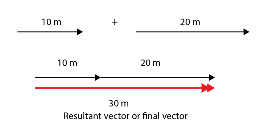
When adding two vectors, such as two displacement vectors \(\vec s_1+ \vec s_2\), the vectors are joined head to tail.
The tail of the second vector joins the head of the first vector.
The resultant vector or final vector spans from the tail of the first vector to the head of the second vector.
For example: (10 m right) + (20 m right) = (30 m right)
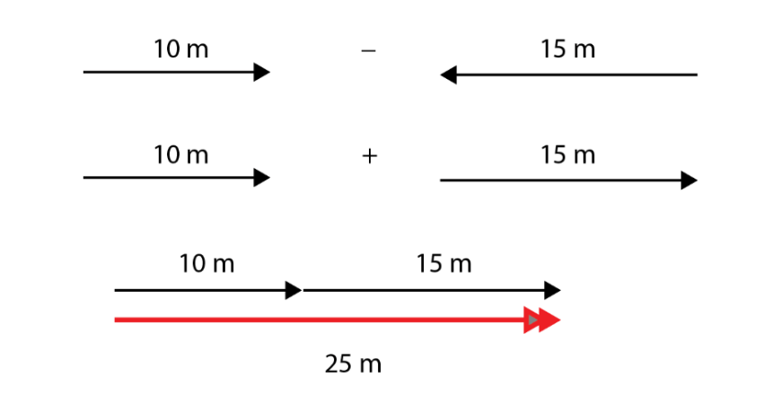
The vector subtraction \(\vec s_1- \vec s_2\) is equivalent to the vector addition \(\vec s_1+ (-\vec s_2)\).
The negative sign reverses the direction of \(\vec s_2\).
For example: (10 m right) – (15 m left) is equivalent to (10 m right) + (-15 m left) = (10 m right) + (15 m right) = (25 m right)
Vectors can also be added and subtracted in two dimensions. We will discuss this in section 3.
A vector can be divided or multiplied by a scalar – for example, displacement is divided by time to get velocity – and the result is another vector in the same direction.
Vector operations beyond those described here are covered in the Year 12 Mathematics Extension courses, and if you continue studying science and maths at university you will frequently use vectors as tools.
If our problem is restricted to motion in a straight line (which can be any line: vertical, horizontal or otherwise, such as the surface of an inclined plane), vectors can only point in one of two directions (e.g. up or down if the line is vertical).
We can solve problems mathematically by designating one direction to be positive and the other to be negative. All vectors that point in the positive direction are then associated with positive numbers, and all vectors pointing in the negative direction correspond to negative numbers.
In particular, when we have a situation involving constant acceleration, the following equations allow us to link acceleration, velocity, displacement and time:
\begin{align*}
v & =u+at\\
s &=ut+\frac{1}{2} at^2 \\
v^2 &=u^2+2as\\
\end{align*}
In these equations, \(u\) represents the object’s initial velocity and \(v\) is its final velocity.
We can also solve problems relating to the relative motion between two objects, or the resultant motion of an object in a moving medium. Consider a situation where an aeroplane is flying on a windy day. Its speed relative to the ground depends on its airspeed but also how fast the air is travelling relative to the ground.
For an object A travelling through a medium B moving relative to the ground G:
\(\vec v_{AG}=\vec v_{AB}+ \vec v_{BG}\)
where \(v_{AG}\) is the velocity of A relative to G
\(v_{AB}\) is the velocity of A relative to B and
\(v_{BG}\) is the velocity of B relative to G.
In other questions, you will know the velocity of both objects relative to the ground and need to calculate their velocity relative to each other. In that case, rearrange the previous equation to find that
\(\vec v_{AB}= \vec v_{AG}- \vec v_{BG}\)
The challenging part of these questions is usually not the vector calculation, which you will have lots of practice with. It’s working out how the information in the question translates into vectors.
Consider the following scenario: a car travelling West at 100 kmh-1 drives past a truck travelling west at 70 kmh-1.
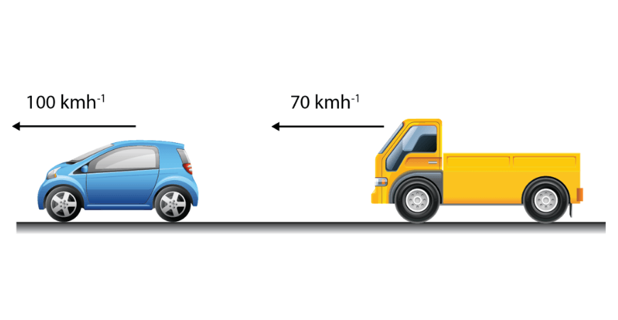
Velocity of the car relative to the ground \(v_{CG}=100 \text{ kmh}^{-1}\) West.
Velocity of the truck relative to the ground: \(v_{CG}=70 \text{ kmh}^{-1}\) West.
Velocity of the car relative to the truck \(v_{CT}=v_{CG}-v_{TG}=30 \text{ kmh}^{-1}\) West.
Across all the sciences, graphs are used to summarise and convey information. Physics is no exception. If we have data about the displacement, velocity or acceleration of an object over time, we can convert it to a graph.
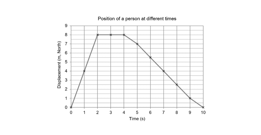
What does this graph tell us? The person starts at some origin point, then travels \(8 \text{ m}\) to the North. Once there, she stays in place for two seconds, before starting to walk back towards the origin. At \(t = 10 \text{ s}\), she is back in her original position.
We can do more than plot and read graphs. There is additional information available through analysing their features. For example, we have established that velocity is the rate of change of displacement. Therefore, if we take the gradient of a displacement-time graph, it represents the quantity \(\frac{Δ\vec s}{Δt}\) which is equal to the instantaneous velocity. Similarly, we can take the gradient of a velocity-time graph to find the instantaneous acceleration.
One more thing we can do with a velocity-time graph is work the other way to calculate total displacement. This is found by taking the area under the graph: any area above the x-axis adds to the total positive displacement, and any area under the x-axis adds to the negative displacement.
More generally, we want to be able to solve problems in two dimensions. Fortunately, most of our techniques remain the same. We just need to extend our understanding of vector operations first.
Adding vectors still works the same way: when adding two vectors, the vectors are joined head to tail. The resultant vector spans from the tail of the first vector all the way to the end of the final vector.
If the problem forms a triangle, you may be able to solve for unknown lengths and angles using the cosine and/or sine rules. More generally, especially if you are adding three or more vectors, the best option is to decompose each vector into horizontal and vertical components using trigonometry:
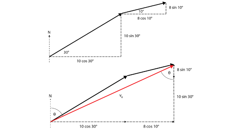
After decomposing, you can add the horizontal components separately, and also the vertical components separately to get the horizontal and vertical components of the final vector. Adding these results in a right angle triangle which you can solve to find the final vector.
There are a few ways to express answers when working in 2D. The most common are compass bearings (e.g. N30E) or true bearings (e.g. 030 T) which you should be familiar with from junior Geography. A word of caution: if you have used the cosine and sine rules to solve for the properties of the unknown vector, the angles inside the triangle are most likely not the angles you need to express your answer.
Almost everything we were able to do in 1D can be expanded to include 2D motion. The process of calculating relative and resultant velocities is the same – the vector operations are simply done in two dimensions instead of one. The equations of motion with constant acceleration can’t be used directly, but in Year 12 you will learn how to modify them to solve further motion problems.
The extra dimension also introduces an extra step to representing motion with graphs. There are now two coordinates that can change with time, and so to fully describe motion we must keep track of both. There are two possibilities: either we keep track of the \(x\) and \(y\) components motion over time, or we describe the vectors by their magnitude \(r\) and bearing \(θ\).
Imagine a car travelling at constant speed around a roundabout:
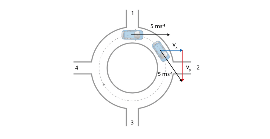
We could represent its motion like this:
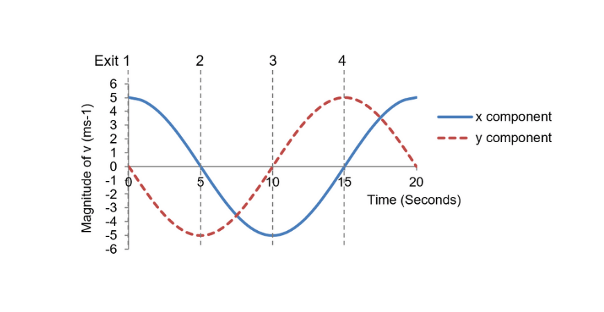
or like this:
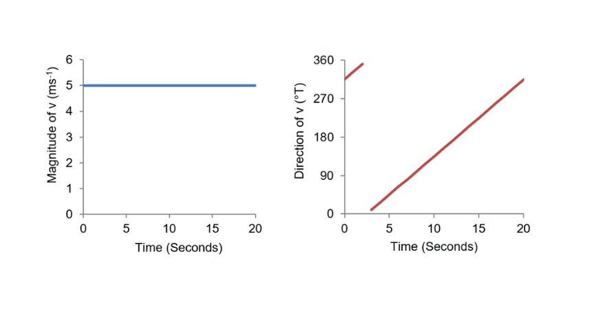
Both sets of plots contain the same information.
Kinematics may not initially seem hugely exciting, but it forms the foundation of our ability to describe everything from atoms to the universe. Once you master this module, you will find it easier to pick up and understand new physics, starting with Module 2: Dynamics.
© Matrix Education and www.matrix.edu.au, 2025. Unauthorised use and/or duplication of this material without express and written permission from this site’s author and/or owner is strictly prohibited. Excerpts and links may be used, provided that full and clear credit is given to Matrix Education and www.matrix.edu.au with appropriate and specific direction to the original content.