Welcome to Matrix Education
To ensure we are showing you the most relevant content, please select your location below.
Select a year to see courses
Select a year to see available courses
Struggling to get on top Maths Standard 2 Algebra? Need to get out of the Band 3/4 doldrums? Well in this part of our Beginner’s Guide to Maths Standard 2, we give you an introduction to Algebra so you can get ahead of your peers!
A worksheet to test your knowledge. 
Free Y12 Maths Std2 Algebra Download
Algebra is an important area of Maths that will allow students to apply what they learn in the HSC to a wide range of real-world problems. Understanding how different variables affect each other is an important logical thinking skill and can be used in everyday life.
For example, using graphical techniques to solve harder algebraic equations makes it more intuitive it is easy to understand the relationships through the visual representation of the curve.
Students should have a strong understanding of basic mathematical operators such as addition, subtraction, multiplication and division.
Students should familiarise themselves with variables and unknown pronumerals, as we will be delving deeper into algebraic expressions throughout this article.
Now we’ll look at the key techniques of substituting values, solving algebraic equations, and changing the subject of a formula.
An algebraic expression is a mathematical expression that contains constant numbers, variables and operations.
The value of an algebraic expression can be found if the value of the pronumeral is known. The process of replacing pronumerals with a known value is called “substitution”.
Given that \(a=3\) and \(b=-4\), find the value of \(2a-2b+2\).
First, we substitute \(a=3\) and \(b=-4\) into the expression and then simplify.
\begin{align*}
2a-2b+2 &=2(3)-2(-4)+2\\
&=6+8+2\\
&=16\\
\end{align*}
Given that \(a=1, b=-4\) and \(c=-2\), find the value of \(b^2-4ac\).Again, we substitute the values into the expression taking caution with the square operator.
\begin{align*}
b^2-4ac&=(-4)^2-4(1)(-2)
&=16+8
&=24
\end{align*}
An equation is solved when a value of the variable is found that satisfies the equation.
The 2 key points in solving an equation are:
Solve the equation \(3x+9=27\).
First, subtract the \(9\) from both sides.
\begin{align*}
3x+9-9&=27-9\\
3x&=18\\
\end{align*}
Now, divide both sides by \(3\) to isolate the variable.
\begin{align*}
\frac{3x}{3} &= \frac{18}{3x} \\
&=6 \\
\end{align*}
Solve the equation \(5(2x-5)=25\).
Dividing both sides by \(5\) we get
\begin{align*}
\frac{5(2x-5)}{5} &= \frac{25}{5}\\
2x-5 &= 5\\
\end{align*}
Now, adding \(5\) to both sides and dividing both sides by \(2\), we solve the equation.
\begin{align*}
2x-5+5 &= 5+5\\
2x &=10\\
\frac{2x}{2} & = \frac{10}{2}\\
x& =5\\
\end{align*}
A formula is an equation that provides the relation between 2 or more pronumerals. The pronumeral that occurs by itself on the left-hand side of the formula is known as the ‘subject’. The subject of a formula can be changed by applying inverse operations and isolating the pronumeral, similar to solving algebraic equations.
Make x the subject of \(y=-2x+8\).
Apply inverse operations to move the x to the left-hand side. In this case, we first subtract 8 from both sides and then divide both sides by \(-2\).
\begin{align*}
y-8&=-2x+8-8\\
&=-2x\\
\frac{y-8}{-2}&=\frac{-2x}{-2}\\
\frac{-y}{2+4}&=x\\
∴x&=\frac{-y}{2+4}\\
\end{align*}
Make a the subject of \(A=\frac{1}{2} h(a+b)\).
\begin{align*}
2A&=2 \left[\frac{1}{2} h(a+b)\right]\\
&=h(a+b)\\
\frac{2A}{h}=\frac{h(a+b)}{h}\\
&=a+b\\
\frac{2A}{h}-b&=a\\
∴a&=\frac{2A}{h}-b\\
\end{align*}
Now we’ll look at Linear Relationships. We’re going to discuss Linear Functions and how to find Linear Functions knowing two points.
A linear function is a function whose graph is a straight line that shows a relationship between two variables, \(x\) and \(y\). Straight lines are typically in the form:
\(y=mx+b\)
Where, \(m\) is the gradient, \(b\) is the y-intercept, \(x\) and \(y\) are variables.
The y-intercept is the point where the graph of a function intersects the y-axis. Similarly, the x-intercept would be the point where the function intersects x-axis.
The gradient is the number that represents the slope or steepness of the line. A larger gradient means a steeper line. The gradient of a line can be calculated by dividing the vertical rise by the horizontal run of the line:
\(m=\frac{rise}{run}=\frac{\text{change in }y}{\text{change in }x}\)
What is the gradient and y-intercept of \(y=2x+4\).
Noting that the straight line can be written in the form \(y=mx+b\), we simply match the gradient and y-intercept components. Therefore, the gradient is \(2\) (i.e. \(m=2\)) and the y-intercept is \(4\) (i.e. \(b=4\)).
What is the gradient and y-intercept of \(y+3x-5=0\).Rewrite the function in the form \(y=mx+b\) by making \(y\) the subject.
\begin{align*}
y+3x-5-3x+5&=0-3x+5\\
y&=-3x+5\\
\end{align*}
Therefore, the gradient is \(-3\) (i.e. \(m=-3\)) and the y-intercept is \(5\) (i.e. \(b=5\)).
To find the equation of a line given the coordinates of two points, we first need to find the gradient. Recall that the gradient can be calculated by:
\( m=\frac{\text{change in }y}{\text{change in }x}\)Given two points, \(A(x_1,y_1 )\) and \(B(x_2,y_2 )\)
\begin{align*}
\text{change in }y&=y_2-y_1\\
\text{change in }x&=x_2-x_1\\
∴m=\frac{\text{change in }y}{\text{change in }x} &=\frac{y_2-y_1}{x_2-x_1 }
\end{align*}
Once the gradient (\(m\)) has been calculated, we can find the value of the y-intercept (\(b\)) by substituting any of the two points into the equation \(y=mx+b\).
Find the equation of the line that passes through (\(1,12\)) and (\(-1,2\)).
First, calculate the gradient between the two points
\begin{align*}
m&=\frac{y_2-y_1}{x_2-x_1 }
&=\frac{2-12}{-1-1}\\
&=\frac{-10}{-2}\\
&=5\\
\end{align*}
Writing the equation in the form \(y=mx+b\).
\(y=5x+b\)
Now, substitute any of the two points into the equation to find \(b\). Let us substitute (\(1,12\)) into the equation.
\begin{align*}
12&=5(1)+b\\
&=5+b\\
∴b&=7\\
\end{align*}
Finally, we express the answer in the form \(y=mx+b\).
\(∴y=5x+7\)
Find the equation of the line with an x-intercept of \(5\) and y-intercept of \(10\).
The x-intercept can be written as (\(0,5\)) and the y-intercept can be written as (\(10,0\)). Therefore, the two points we will be using are (\(0,5\)) and (\(10,0\)). Hence, gradient is
\begin{align*}
m&=\frac{y_2-y_1}{x_2-x_1}\\
&=\frac{0-10}{5-0}\\
&=\frac{-10}{5}\\
&=-2
\end{align*}
The equation is in the form \(y=-2x+b\). Recalling the fact that \(b\) is the y-intercept, we know that \(b=10\) from the question. Therefore, the equation is \(y=-2x+10\).
In the past section, you saw examples with a single equation, but there are many problems which can only be solved by considering multiple equations. When we have multiple equations that are connected to each other we call it a system of equations, which need to be solved simultaneously. There’s no limit on how many equations can be in a system, but in the Standard Maths HSC course, you’ll only need to consider systems with two equations.
There are a few different ways to solve simultaneous equations: graphical, elimination and substitution. The graphical method is the only assessable method in the Standard Maths course, but if you’re interested in the other two there are some examples in our blog post – https://www.matrix.edu.au/beginners-guide-year-9-maths/part-8-simultaneous-equations/.
Example: There are two numbers x and y which add together to make 2, and the difference between y and x is 3. Determine the value of x and y.For this problem the equations haven’t been specified, which highlights the importance of being able to interpret the question and form equations. We get:
Equation 1: \(x + y = 2\)
Equation 2: \(y – x = 3\)
Recall from the previous section that both equations are linear functions and are graphed as a straight line. The solution to this set of simultaneous equations is simply the point where the two straight lines intersect! Solving this question is then done by drawing the lines and reading the coordinates of the intersection point from the x and y axes.
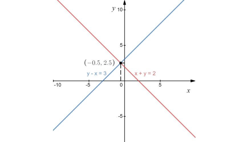
Here the solution is \(x = -0.5, y = 2.5\)
To show what this means, we can test by substituting the solution back into the original equations:
\begin{align*}
-0.5 + 2.5 &= 2\\
2.5 – -0.5 &= 3\\
\end{align*}
This means that we have found the values that satisfy both equations at the same time! As non-parallel straight lines only intersect once, there will only be one possible solution for systems of linear equations. A common application of simultaneous equations is when figuring out revenue and costs for a business/event.
Example: Chris wants to hold a movie screening as a fundraiser. He needs to hire a projector for \($150\) and will be providing food and drinks worth \($3\) to everyone with a ticket. He plans to sell the tickets for \($15\). Approximate how many people need to buy tickets for Chris to break even.
The term “break-even” means the point where the cost and revenue are the same so that Chris has a profit/loss of \($0\). For a set of equations describing cost and revenue, this break-even point will be at the intersection of the two lines.
The equations would be:
Equation 1: Cost \(C = 150 + 3n\)
Equation 2: Revenue \(R = 15n\)
Where \(n\) is the number of people who have purchased tickets.
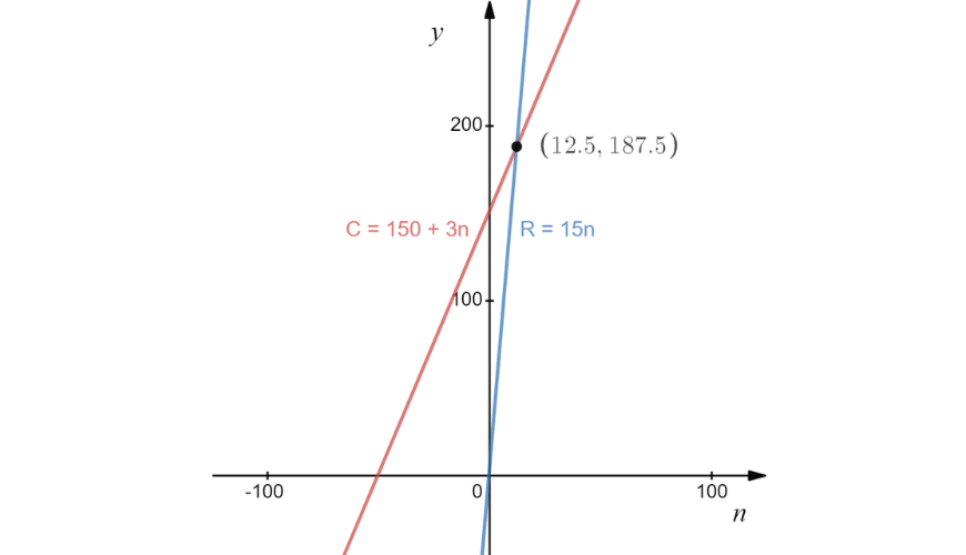
Reading from the axes we find the intersection point at \(n = 12.5, y = 187.5\).
This means that if he sold \(12.5\) tickets he would have received \($187.5\) and spent \($187.5\) for a total of \($0\) (he has broken even). Since it is not possible to sell a half ticket, the answer would be rounded up to \(n = 13\) tickets required to break even. Less than \(13\) tickets would mean that Chris loses money, and above \(13\) tickets he will have more revenue to give to the charity.
Recall that a linear relationship is an equation that can be graphed as a straight line. Real-world problems take many different forms, and a straight line is often not sufficient to describe a situation. In this section, we’ll explore the three different kinds of non-linear relationships. When we use one of these relationships to describe a problem, we call it a model.
An exponential function is a constant raised to the power of x, with the following form:
\(y=a^x\)
As the \(x\) value increases, the constant is raised to a higher power and so the \(y\) value grows very quickly. This is called “exponential growth”, a term you may have heard being used to describe population growth or interest in finance. The \(x\) value may also be negative, which means that the y value would be decreasing, or “decaying”. We will only be considering positive values of \(a\).
Any number to the power of \(0\) is equal to \(1\), so the exponential curve will always pass through the point (\(0,1\)) regardless of a value! We are only considering positive \(a\) values, so the curve will always be positive. With \(a > 1\):
\(a^x\) will be an increasing curve
\(a^x\) will be a decreasing curve
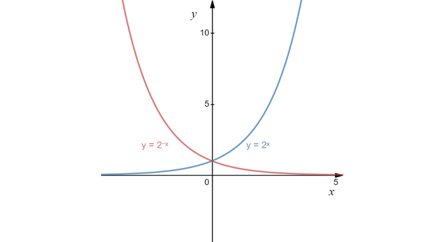
You’ve probably noticed how the curve goes towards the x axis, but it’s important to note that the y value never actually reaches \(0\)!
We call the x axis an asymptote of the curve, which is a line that it gets closer and closer to but never touches. Special Case for \(0 < a < 1\):
Sometimes you may have a value of a which is less than 1, and this results in a curve in the opposite direction, i.e. for \(a^x\), the curve will be decreasing and for \(a^x\) the curve will be increasing.
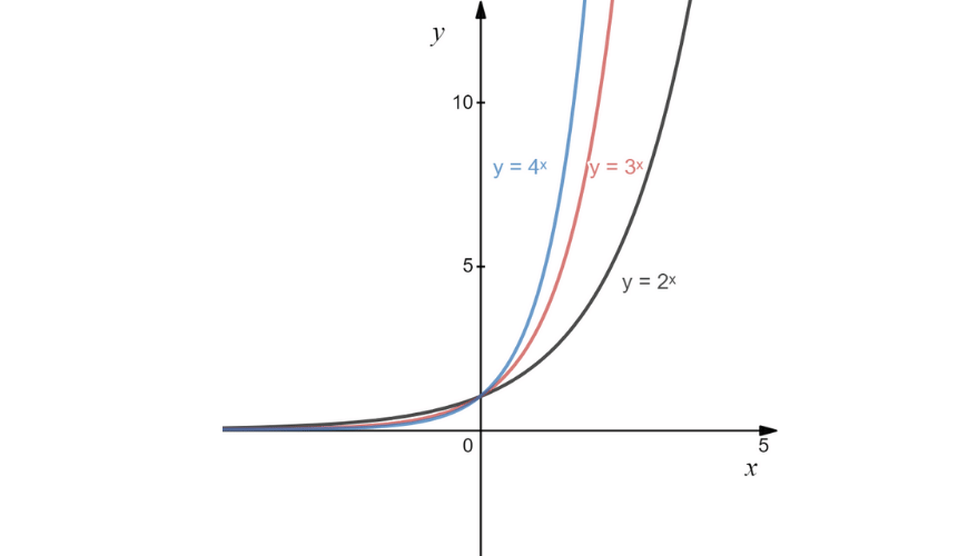
The value of \(a\) changes how fast the curve increases or decreases, which when graphed will change how steep it is.
Plot the exponential curve \(2^{(-x)} \) and approximate the x value at \(y = 3\). The first step is to fill in a table of values:
| \(x\) | \(-2\) | \(-1.5\) | \(-1\) | \(-0.5\) | \(0\) | \(0.5\) | \(1\) |
| \(y\) | \(4\) | \(2.83\) | \(2\) | \(1.41\) | \(1\) | \(0.71\) | \(0.5\) |
We can now plot the curve by joining these points to form the shape of the exponential curve.
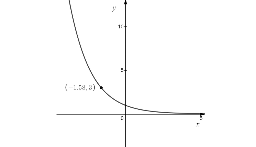
The x value at \(y = 3\) can be found by reading it off the x-axis, which is around \(x = 1.6\).
A quadratic function is an equation which has a power of \(x^{2}\), with the general form \(y = ax^2 + bx + c\).
The simplest parabola is \(y = ax^2\). There are a few special terms that we use to describe the shape of a parabola:
The vertex is the point where the curve changes direction. The axis of symmetry is the x value of the vertex. The concavity describes whether the curve us shaped like a smile or a frown (concave up or concave down). The x intercepts are the points where the curve touches the x axis. The y intercept is the point where the cure touches the y axis.
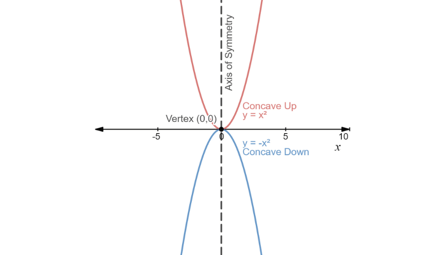
As with the exponential function, the value of a determines how steep the curve is. For a parabola, this changes how “thin” the curve looks, with a high value of a being a thin curve and a low value of a being a wide curve.
Often there will be a second constant in the equation, such that it has the form \(y = ax^2 + b\). This \(b\) value will move the curve either up or down.
Plot the curve \(y = 0.5x^2\) and find the positive value of x for \(y = 3\). We again draw a table of values, then join the points to form the shape of a parabola.
| \(x\) | \(-3\) | \(-2\) | \(-1\) | \(-0\) | \(1\) | \(2\) | \(3\) |
| \(y\) | \(4.5\) | \(2\) | \(0.5\) | \(0\) | \(0.5\) | \(2\) | \(4.5\) |
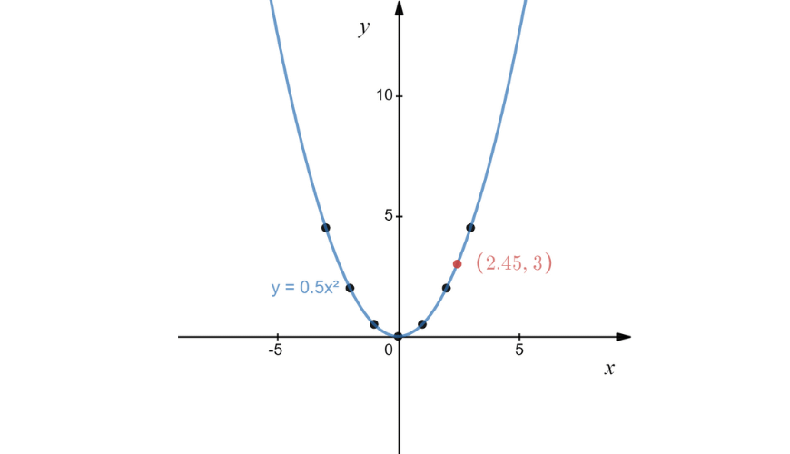
From looking at the curve and reading the axes, the x value for \(y = 3\) is around \(2.5\).
A common problem which uses a quadratic model is the stopping distance for a car, which is how far a driver travels after noticing an obstacle and beginning to stop.
There are two terms in the equation, the reaction distance and stopping distance. The reaction distance is the distance travelled before the driver starts braking, and the braking distance is how far the car travels depending on the type of surface, car weight etc. Mathematically this is:
\(d=\frac{5vt}{18}+{v^2}{170}\)Where:
\(d\) is the stopping distance (metres)
\(v\) is the velocity of the car before braking (km/h)
\(t\) is the reaction time of the driver (seconds).
To find stopping distance all you need to do is substitute in the \(v\) and \(t\) values.
To find the velocity for a certain stopping distance, you would need to plot the curve and read from the axes.
In many real-world examples such as stopping distance, we only consider positive x values, so it is only necessary to plot that half of the curve. This makes sense as if the velocity was less than \(0\), the car would be travelling backwards.
The final type of non-linear function we’ll be considering is the reciprocal function, which has \(x\) in the denominator:
\(y=\frac{k}{x}\)Where \(k\) is a constant. The shape of the graph of this equation is called a hyperbola.
This is a special curve as it is divided into two separate sections! For a positive k-value the arms are in the 1st and 3rd quadrant (top right and bottom left), and a negative k-value in the 2nd and 4th quadrant (top left and bottom right).
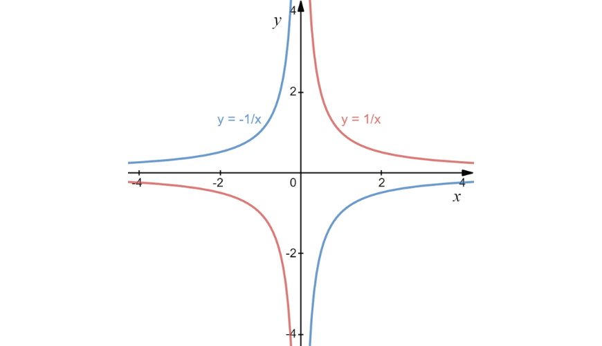
An important feature to note is that a hyperbola has two asymptotes, the x and y axis. The value of x cannot be zero, as this would be a division by zero and is undefined. The procedure for graphing this equation is the same as the previous non-linear functions, simply complete a table of values and then connect them in the shape of a hyperbola.
A group of students are planning a laser tag event in the holidays, and the price per person is less if more people attend.
This can be modelled by \(C = \frac{500}{n}\), where \(C\) is the cost per person and \(n\) is the number of people. Sketch the curve and determine how many people need to attend for it to cost \($25\) each. As this is a situation where only positive values of \(n\) would make sense (you can’t have a negative number of people!), only the positive half of the curve needs to be drawn.
| \(n\) | \(5\) | \(7.5\) | \(10\) | \(15\) | \(17.5\) |
| \(C\) | \(100\) | \(66.67\) | \(50\) | \(33.33\) | \(28.57\) |
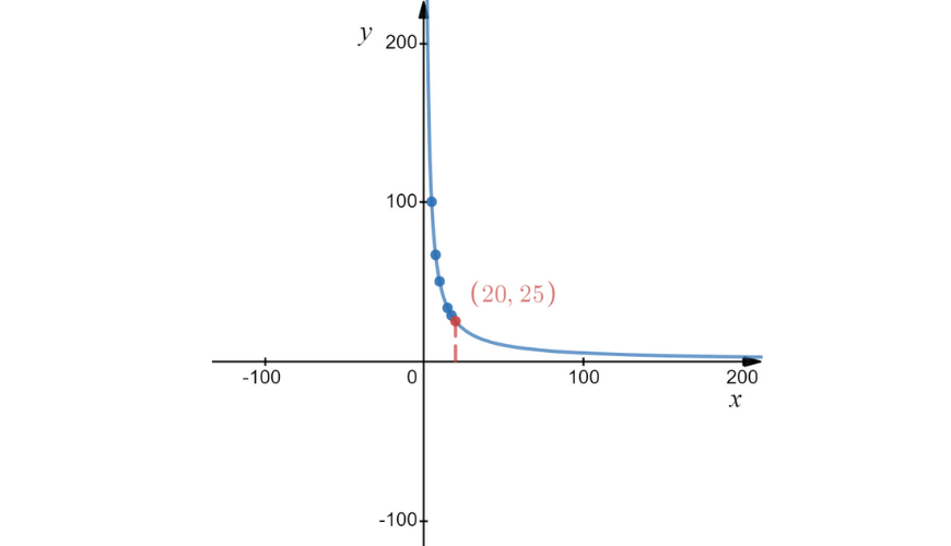
Although the number of people for a cost of \($25\) can be read from the graph, for reciprocal functions it is simple to find the result algebraically.
We have \(C = 25\), so:
\(25=\frac{500}{n} ⟶ 500=25n ⟶ n=\frac{500}{25}=20\)
1. Consider the function \(C=5N-\frac{1}{3} x\).
2. Solve the equation \(7(7x-7)=77.3\).
3. Find the equation of the line that passes through (\(2,21\)) and (\(-4,-27\)).
4. Two numbers x and y add together to \(5\), and the difference between y and x is \(1.5\). Determine the values of x and y (by drawing a graph or otherwise).
5. Find the \(x\) value at \(y = \frac{1}{3}\) for \(y=\frac{-2}{x6}\). Identify the vertex, axis of symmetry, x and y intercepts and minimum value for the following parabola
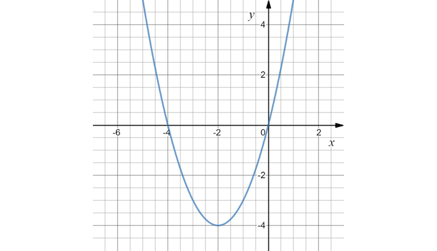
6. Identify the vertex, axis of symmetry, x and y intercepts and minimum value for the following parabola
7. James is travelling down the highway at \(110\) km/h and has a reaction time of \(0.75\)s. Calculate the stopping distance.
1.
2. \(x=\frac{18}{73}\).
3. \(y=8x+54\).
4. Equations are \(x + y = 5\) and \(y – x = 2\).
The solution is \(x = 1.5,y = 3.5\)
5. \(x = -6\)
6. Vertex is (\(-2,-4\))
Axis of symmetry is \(x = -2\)
x-intercepts are (\(-4,0\)) and (\(0,0\))
y-intercept is (\(0,0\))
Minimum value = \(-4\)
7. \(d=\frac{5×0.75×110}{18}+\frac{110^2}{170}=94m\)
© Matrix Education and www.matrix.edu.au, 2025. Unauthorised use and/or duplication of this material without express and written permission from this site’s author and/or owner is strictly prohibited. Excerpts and links may be used, provided that full and clear credit is given to Matrix Education and www.matrix.edu.au with appropriate and specific direction to the original content.